Making Connections
We continue our experimentation of the data for the Chicago Transit Authority (CTA). First, we scan the downloaded files and look for connections using a plain Python dictionary as data structure. Building a dictionary from scratch is costly and in the second stage we use mysql tables to compute connections. We conclude with a plot of the adjacency matrix of the CTA stops and connections.
CTA Tables
Recall from the last lecture that every file in the General Transit Feed Specification (GTFS) is a comma separated value text file, which represents a table in a relational database.
We will store the connections between stops in a dictionary.
The file stop_times.txt has lines
22043803629,07:38:30,07:38:30,30085,22,"UIC",0,98455
22043803629,07:40:30,07:40:30,30069,23,"UIC",0,100813
These two lines stat that stops 30085 ("Clinton-Blue")
and 30069 ("UIC-Halsted") are connected via stop head sign "UIC".
In a dictionary D we store D[(30085,30069)] = "UIC".
The initialization and start of the loop
in the script ctaconnections.py are listed below.
FILENAME = 'CTA/stop_times.txt'
print 'opening', FILENAME, '...'
DATAFILE = open(FILENAME, 'r')
COUNT = 0
PREV_STOP = -1
PREV_HEAD = ''
D = {}
while True:
    LINE = DATAFILE.readline()
    if LINE == '':
        break
    L = LINE.split(',')
The line L contains the data read from file.
From the example above, observe that the stop id
is in L[3] and the head sign is in L[5].
# continuation of the while True loop
    try:
        (STOP, HEAD) = (int(L[3]), L[5])
        if PREV_STOP == -1:
            (PREV_STOP, PREV_STOP) = (STOP, HEAD)
        else:
            if PREV_HEAD == HEAD:
                D[(PREV_STOP, STOP)] = HEAD
            else:
                (PREV_STOP, PREV_HEAD) = (STOP, HEAD)
    except:
        print 'skipping line', COUNT
    COUNT = COUNT + 1
print D, len(D)
There are 11,430 lines in stops.txt.
Except for the first line, every line is stop.
Viewing each stop as a node in a graph,
there are 11,429 nodes.
The adjacency matrix has 11,429 rows and 11,429 colums
or 130,622,041 elements.
The dictionary stores 583,279 elements, less than 0.5%
of the total possible \(11,429 \times 11,429\) elements.
CTA Schedules
The problem is to compute connections between the stops. An example session could run as follows.
$ python3 ctaconnectstops.py
opening CTA/stop_times.txt ...
loading a big file, be patient ...
skipping line 0
573036 connections
give start stop id : 30085
  give end stop id : 30069
30085 and 30069 are connected by "UIC"
The documentation string for the function to build a dictionary is listed below.
FILENAME = 'CTA/stop_times.txt'

def stopdict(name):
    """
    Opens the file with given name.
    The file contains scheduled arrival and departure times
    for each stop on each trip.
    On return is a dictionary D with keys (i,j) and strings
    as values, where i and j are stop ids and the value is
    the empty string if i and j are not connected by a trip,
    otherwise D[(i,j)] contains the trip name.
    """
The function main() in the script ctaconnectstops.py
is as follows.
def main():
    """
    Creates a dictionary from the file
    stop_times.txt and prompts the user
    for a start and end stop id.
    The result of the dictonary query
    tells whether the stops are connected.
    """
    conn = stopdict(FILENAME)
    print len(conn), 'connections'
    i = input('give start stop id : ')
    j = input('  give end stop id : ')
    outs = str(i) + ' and ' + str(j)
    if not conn.has_key((i, j)):
        print outs + ' are not connected'
    else:
        print outs + ' are connected by ' + conn[(i, j)]
Instead of a dictionary, we can represent the graph of connections
between the stops with a sparse matrix.
The package scipy provides the package sparse
to work with sparse matrices.
>>> from scipy import sparse
To store an adjacency matrix similar to D[(i,j)]
we use the COOrdinate format:
>>> from scipy import array
>>> from scipy.sparse import coo_matrix
>>> row = array([0,3,1,0])
>>> col = array([0,3,1,2])
>>> data = array([4,5,7,9])
>>> A = coo_matrix((data,(row,col)),shape=(4,4))
>>> A.todense()
matrix([[4, 0, 9, 0],
        [0, 7, 0, 0],
        [0, 0, 0, 0],
        [0, 0, 0, 5]])
We can compute with matrices, as illustrated
in the continuation of the session with scipy below.
>>> B = A*A
>>> B.todense()
matrix([[16,  0, 36,  0],
        [ 0, 49,  0,  0],
        [ 0,  0,  0,  0],
        [ 0,  0,  0, 25]])
An adjacency matrices \(A\) has the following propoerty: if \((A^k)_{i,j} \not=0\), then nodes \(i\) and \(j\) are connected by a path of length \(k\).
An alternative way to define a sparse matrix in scipy
is via a dictionary of keys:
dok_matrix is a dictionary of keys based sparse matrix.
It allows for efficient access of individual elements
and can be efficiently converted to a coo_matrix.
Consider the session below.
>>> from scipy import sparse
>>> A = sparse.dok_matrix((4,4))
>>> A[1,2] = 1
>>> B = sparse.coo_matrix(A)
>>> B.todense()
matrix([[ 0.,  0.,  0.,  0.],
        [ 0.,  0.,  1.,  0.],
        [ 0.,  0.,  0.,  0.],
        [ 0.,  0.,  0.,  0.]])
>>> B.todense()
matrix([[ 0.,  0.,  0.,  0.],
        [ 0.,  0.,  1.,  0.],
        [ 0.,  0.,  0.,  0.],
        [ 0.,  0.,  0.,  0.]])
>>> B.row
array([1], dtype=int32)
>>> B.col
array([2], dtype=int32)
>>> B.data
array([ 1.])
>>> B.nnz
1
The attributes row, col, data, and nnz
respectively return the row, column indices, the corresponding
data, and the number of nonzeros.
Printing all entries of a large sparse matrix does not give any insight in its sparse structure. In a plot of a sparse matrix, every nonzero element is marked by one dot in the plot. Zero elements in the matrix are left unmarked as white space. An example of a random sparse matrix (with 10% of its entries generated as nonzero elements) is shown in Fig. 100.
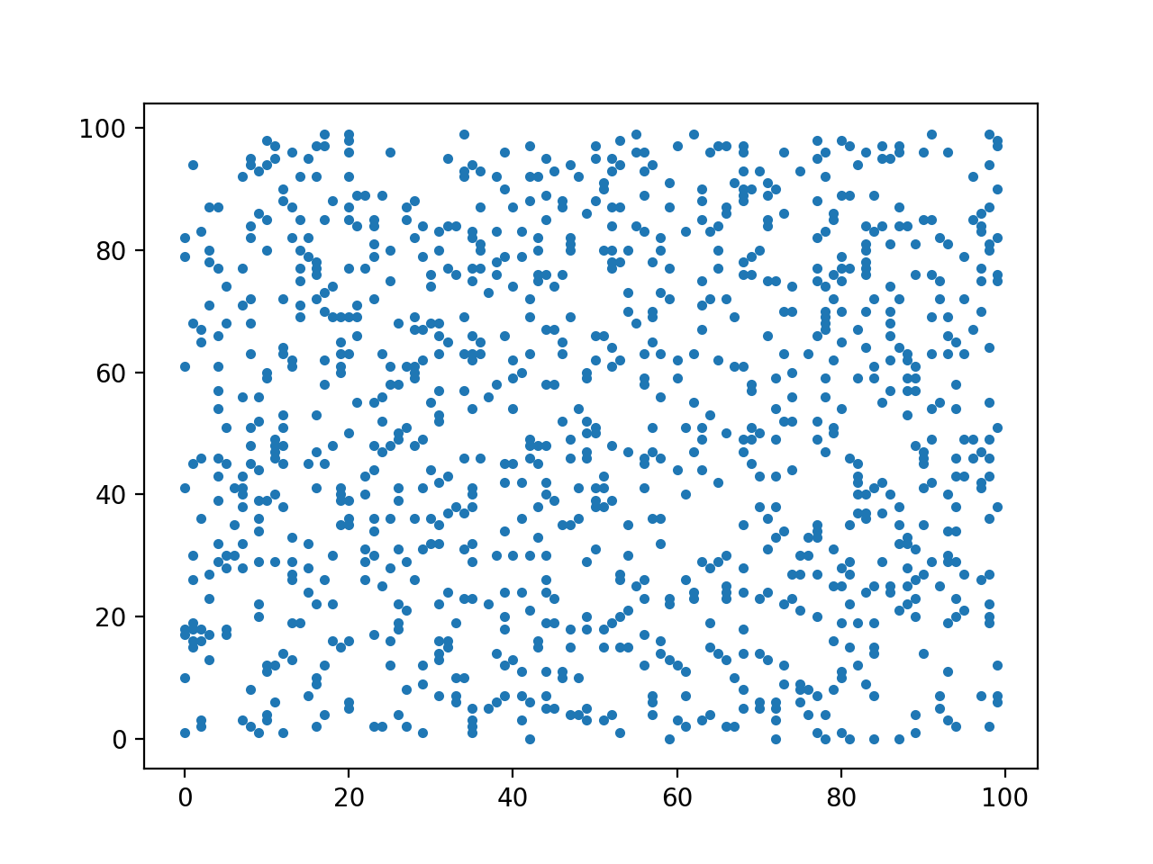
Fig. 100 A spy plot of a sparse matrix.
The script spy_matrixplot.py which uses matplotlib
to produce Fig. 100 is listed below.
import numpy as np
from matplotlib.pyplot import spy
import matplotlib.pyplot as plt
from scipy import sparse

r = 0.1 # ratio of nonzeroes
n = 100 # dimension of the matrix
A = np.random.rand(n,n)
A = np.matrix(A < r,int)
S = sparse.coo_matrix(A)
x = S.row; y = S.col
fig = plt.figure()
ax  = fig.add_subplot(111)
ax.plot(x,y,'.')
plt.show()
The matrix plot for the CTA connections is in Fig. 101.
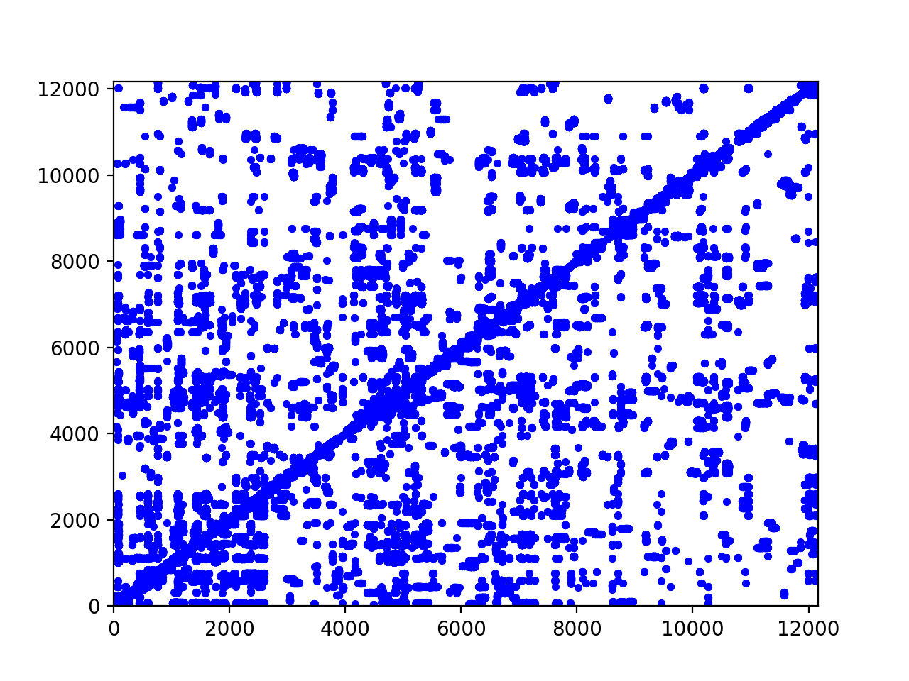
Fig. 101 The spy plot for the connections of the CTA.
The adjacency matrix plotted in Fig. 101
is computed with the script ctamatrixplot.py listed below.
"""
This script creates a sparse matrix A,
which is the adjacency matrix of the stops:
A[i,j] = 1 if stops i and j are connected.
"""
from scipy import sparse
import matplotlib.pyplot as plt

filename = 'CTA/stop_times.txt'
print 'opening', filename, '...'
file = open(filename,'r')

n = 12165
A = sparse.dok_matrix((n,n))
i = 0; prev_id = -1; prev_hd = ''
while True:
    d = file.readline()
    if d == '': break
    L = d.split(',')
    try:
        id = int(L[3]); hd = L[5]
        if prev_id == -1:
             (prev_id, prev_hd) = (id, hd)
        else:
             if prev_hd == hd:
                 A[prev_id, id] = 1
             else:
                 (prev_id, prev_hd) = (id, hd)
    except:
        pass # print 'skipping line', i
    i = i + 1
B = sparse.coo_matrix(A)
x = B.row; y = B.col
fig = plt.figure()
ax  = fig.add_subplot(111)
ax.set_xlim(-1,n)
ax.set_ylim(-1,n)
ax.plot(x,y,'b.')
plt.show()
Adjacency Matrices
A matrix is a 2-dimensional table of numbers,
indexed by rows and columns.
An adjacency matrix A is a matrix of zeroes and ones:
A[row][column] = 1: row and column are connected,A[row][column] = 0: row and column are not connected.
For example, the matrix
1 0 1 0 0
0 1 1 0 1
0 0 0 0 0
1 0 1 0 1
0 1 1 1 0
was generated by the script
from random import randint

def random_adjacencies(dim):
    """
    Returns D, a dictionary of dictionaries to
    represent a square matrix of dimension dim.
    D[row][column] is a random bit.
    """
    result = {}
    for row in range(dim):
        result[row] = {}
        for column in range(dim):
            result[row][column] = randint(0, 1)
    return result
The matrix is represented by D, as a dictionary of dictionaries,
as D[row] is again a dictionary with the elements on row
indexed by keys we call column.
The writing of a matrix is defined by the the function write.
def write(dim, mat):
    """
    Writes the square matrix of dimension dim
    represented by the dictionary mat.
    """
    for row in range(dim):
        for column in range(dim):
            print(' %d' % mat[row][column], end='')
        print('')
In the random_adjacencies we also store the zero elements.
The sparse representation omits storing the zeroes.
When looking for connections, we search the adjacency matrix. Consider again the example:
1 0 1 0 0
0 1 1 0 1
0 0 0 0 0
1 0 1 0 1
0 1 1 1 0
Observe the following:
- There is no direct path from 1 to 3.
- We can go from 1 to 4 and from 4 to 3.
We can answer the question whether there exists a path between two nodes via one intermediate node with a matrix-matrix multiplication, as illustrated below.
>>> import numpy as np
>>> A = np.matrix([[1, 0, 1, 0, 0],
... [0, 1, 1, 0, 1],
... [0, 0, 0, 0, 0],
... [1, 0, 1, 0, 1],
... [0, 1, 1, 1, 0]])
>>> A*A
matrix([[1, 0, 1, 0, 0],
        [0, 2, 2, 1, 1],
        [0, 0, 0, 0, 0],
        [1, 1, 2, 1, 0],
        [1, 1, 2, 0, 2]])
>>> _[1, 3]
1
\(A^2_{i, j} = 1\) means there is a path from \(i\) to \(j\) with one intermediate stop.
The main program to search a random adjacency matrix follows.
def main():
    """
    Prompts the user for the dimension
    ans shows a random adjacency matrix.
    """
    dim = int(input('Give the dimension : '))
    mtx = random_adjacencies(dim)
    write(dim, mtx)
    src = int(input('Give the source : '))
    dst = int(input('Give the destination : '))
    mxt = int(input('Give the maximum number of steps : '))
    pth = search(dim, mtx, dst, 0, mxt, [src])
    print('the path :', pth)
The recursive search function is defined below.
def search(dim, mat, destination, level, maxsteps, accu):
    """
    Searchs the matrix mat of dimension dim for a path
    between source and destination with no more than
    maxsteps intermediate stops.
    The path is accumulated in accu, initialized with source.
    """
    source = accu[-1]
    if mat[source][destination] == 1:
        return accu + [destination]
    else:
        if level < maxsteps:
            for k in range(dim):
                if k not in accu:
                    if mat[source][k] == 1:
                        path = search(dim, mat, destination, level+1, \
                                      maxsteps, accu + [k])
                        if path[-1] == destination:
                            return path
        return accu
Exercises
- Modify
ctastopname.pyso the user is prompted for a string instead of a number. The modified script prints all id’s and corresponding names that have the given string as substring. - Instead of using numpy and scipy, use turtle to draw the spy plot of a matrix.
- Instead of using numpy and scipy, use the canvas widget of tkinter to draw the spy plot of a matrix.
- Apply the
searchto work on the adjacency matrix of the data obtained for the CTA.