Lecture 2: the notebook – structuring and documenting work flow

We can use the notebook as a calculator or as a computer program, but such use does not take the full advantage of all capabilities of the notebook. The SageMath project is separate from the Jupyter project [KRPetal16].

If you compiled SageMath from source, then you are likely starting in a Terminal window. To launch the program with a Jupyter notebook, type

sage --notebook='ipython'

at the command prompt in a Terminal window.

the Jupyter notebook in CoCalc

To use the Jupyter notebook in CoCalc, in the creation of a new file, choose for the Jupyter notebook among the Select the type options, see Fig. 2.

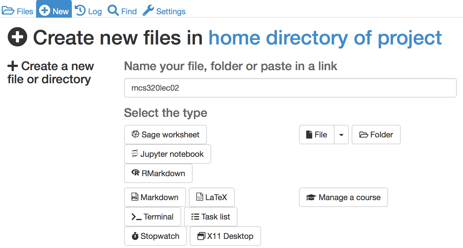
Fig. 2 Selecting the Jupyter notebook in CoCalc.

Jupyter notebooks are stored in files with the extension ipynb. In the CoCalc environment, to save a notebook to a file on your computer, select the first Notebook (.ipynb)... option of the Download as... menu of the File menu, available at the top left corner, see Fig. 3.

Be aware that many browsers will (sometimes by default) add the extension .txt to the downloaded file, which then causes problems when loading the downloaded file in a SageMath session or when uploading to the cloud.

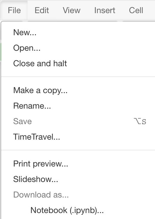
Fig. 3 Saving a Jupyter notebook in CoCalc onto your computer.

Note the Print preview... option, shown in the menu in Fig. 3. Selecting this option converts the notebook into an HTML file. The HTML file can then be printed, just as you would print out any web page in your browser.

The opposite to a download is an upload, useful if we want to bring a Jupyter notebook from our computer into CoCalc. To upload, click on the Upload button, shown at the the top right in Fig. 4.

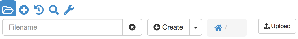
Fig. 4 The upload button to upload a Jupyter notebook from your computer.

Formatting a Notebook

By default, all cells are of type Code and contain instructions for SageMath to execute, as if at the command prompt or as in a script.

To introduce structure in a notebook, we can add section headings. Suppose we would want to place the title Computing with Symbols at the start of our notebook.

1. Insert a new cell before the first cell in the notebook, via the Insert Cell Above available from the dropdown Insert menu at the top of the notebook.

2. Instead of the Code, we select Heading as the type of the cell. The type of the cell can be modified via the toolbar of the notebook.

3. Once the type of the cell is changed to Heading, we type in the title Computing with Symbols after the # symbol.

4. Executing the cell displays the formatted title.

To add text, we follow the same steps as before, but select the Markdown type instead of the default Code.

What is between dollar signs ($) will be formatted by LaTeX.
Text between two single opening left quotes (``)
and two single closing left quotes will not be formatted.

Executing the cell displays the formatted text. To see the original unformatted text, select the Raw NBConvert, instead of the default Code.

Exact, Symbolic, and Approximate Computations

We distinguish between three types of computations:

1. An exact computation is free from errors.

   Example: \(\frac{1}{2} + \frac{1}{4} = \frac{3}{4}\).

2. A symbolic computation operates on symbols.

   Example: \(\sin(\pi/3) = \sqrt{3}/2.\)

   Note: \(\sqrt{3}\) is the symbol for the unevaluated function sqrt(3).

3. An approximate computation works in limited precision.

   Example: \(\sin(3.1415/3) = 0.8660.\)

Consider the following computation: Pi10 = pi.n(digits=10)

The Pi10 evaluates to 3.141592654, an approximation for \(\pi\), accurate to 10 decimal places.

The statement delta = pi - Pi10 shows pi - 3.141592654, which is a symbolic expression.

Now consider the following two statements:

1. delta.n(digits=10) evaluates to 0.0000000000

2. delta.n(digits=11) evaluates to 3.6379788071e-12

Which outcome is correct? Well, consider:

1. The 0.0000000000 shows that the expression pi - Pi10 evaluates indeed to zero when the working precision is 10 decimal places.

2. When evaluating pi - Pi10 with 11 decimal places in the working precision, then the error is 3.6379788071e-12.

Both outcomes are correct with regard to the working precision.

Assignments

1. Copy the assignments of the first lecture in the Markdown cells of a Jupyter notebook. Use Exercise 1, Exercise 2, etc as the headers in front of each assignment.

2. Add cells to the Jupyter notebook of the first assignment. Each added cell contains your solution of an exercise.

References

[KRPetal16]

T. Kluyver, B. Ragan-Kelley, F. Pérez, B.Granger, M. Bussonnier, J. Frederic, K. Kelley, J. Hamrick, J. Grout, S. Corlay, P. Ivanov, D. Avila, S. Abdalla, C. Willing, and Jupyter Development Team: Jupyter Notebooks — a publishing format for reproducible computational workflows. In F. Loizides and B. Schmidt, editors, Positioning and Power in Academic Publishing: Players, Agents, and Agendas, pages 87–90. IOS Press, 2016.