Lecture 4: Exact and Floating-Point Numbers
The capability to compute exactly and in high precision is one of the main features of computer algebra. In this lecture we illustrate how to compute exactly with integer and rational numbers, and to compute with multiprecision arithmetic.
We can approximate a transcendental number such as \(\pi\) as a floating-point number up to any number of decimal places. Instead of a floating-point approximation, we may approximate with a continued fraction expansion. In Sage we can compute continued fractions up to a certain number of terms or up to a given number of bits in the precision. The convergents of a continued fraction gives us a sequence of increasingly more accurate rational approximations for \(\pi\). We cover machine precision. Irrational and algebraic numbers are defined. We introduce the reverse operation to computing an approximation of an irrational number. Given an approximation for a number and a tolerance, we may find the smallest polynomial that has this number as a root. For example, with sympy we compute \(\sqrt{2}\) from an approximation for the \(\sqrt{2}\), as \(\sqrt{2}\) is a solution of \(x^2 - 2\).
Integer and Rational Numbers
The division of two integer numbers gives a rational number. Selecting its numerator and denominator is straightforward:
a = 3/4
print type(a)
print numerator(a), denominator(a)
Any irrational or transcendental can be approximated with continued fractions. A continued fraction is defined by a list of natural numbers, which are called convergents. For example:
x = sqrt(2)
c = continued_fraction(x)
print c
show(c)
which prints
[1; 2, 2, 2, 2, 2, 2, 2, 2, 2, 2, 2, 2, 2, 2, 2, 2, 2, 2, 2, ...]
and the output of show(c) is displayed
in Fig. 6.
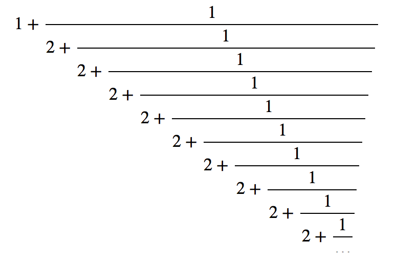
Fig. 6 The continued fraction expansion of \(\sqrt{2}\).
We can verify that
approximates \(\sqrt{2}\) up to 3 correct decimal places:
f = 1 + 1/(2 + 1/(2 + 1/(2 + 1/2)))
print(f)
print(float(f), float(x))
The continued fraction defines convergents which are the consecutive best rational approximations.
c.convergents()
The output is a lazy list which shows only the first three numbers.
To compute the first five convergents, one takes a slice of length 5
and then converts that slice to a list:
v = c.convergents()
v[:5].list()
Each convergent is a rational approximation.
The output of the last command is
[1, 3/2, 7/5, 17/12, 41/29] which is a list of
increasingly more accurate approximations converging
to \(\sqrt{2}.\)
The quickest way to get a rational approximation for the square root of 2, accurate to 2 decimal places, goes as follows
QQ(sqrt(2).n(digits=2))
With a list comprehension, we can then compute the sequence
of increasingly more accurate rational approximations for sqrt(2).
[QQ(sqrt(2).n(digits=k)) for k in range(2,10)]
Observe that this sequence is different from the convergents,
because the list above contains rational approximations with
a prescribed accuracy (of k decimal places), whereas the
convergents give the sequence of the next best rational approximations.
Floating-Point Numbers
The default floating-point type is float as in Python.
The machine precision is defined as the smallest
positive number we can add
to 1.0 and see a difference from 1.0.
A double float has 53 bits in its fraction,
a single float has a fraction of 22 bits long.
We can verify the machine precision calculation with the predefined
constants of the numpy package.
print('machine precision (double float) :', float(2^(-52)))
print('machine precision (single float) :', float(2^(-23)))
import numpy
from numpy import finfo
print(finfo(float).eps)
print(finfo(numpy.float32).eps)
To compute with higher than double precision, we can make a RealField. Since the argument is in bits, we multiply with the number of decimal places we want in our precision with the 2-logarithm of 10. For 50 decimals, we do
nbits = 50*log(10,2)
print('number of bits for 50 decimal places :', int(nbits))
R = RealField(nbits)
print('50-digit approximation of sqrt(2) =', R(x))
We will use this field to verify the accuracy of the convergents calculating in R with a list comprehension
c = continued_fraction(sqrt(2))
v = c.convergents()
a = v[:20].list()
print(['%.2e' % R(sqrt(2)-p) for p in a])
The numbers are displayed in scientific format and we see the exponent gradually decreasing till -15, which indicates that the last convergent is accurate up to 15 decimal places.
A number as \(\sqrt{2}\) is an irrational number.
But it is not a transcendental number
because \(\sqrt{2}\) is a root of \(x^2 - 2 = 0\) and
therefore we say that \(\sqrt{2}\) is an algebraic number.
With the nsimplify of sympy, given an approximation for a root,
we can reconstruct the polynomial and thus find the
closest exact number of the algebraic number.
asqrt2 = numerical_approx(sqrt(2),10)
print(asqrt2)
from sympy import nsimplify
print(nsimplify(asqrt2,tolerance=0.001,full=True))
The last statement prints sqrt(2), obtained from a 10-bit
approximation 1.4 for \(\sqrt{2}\).
Assignments
Explain the outcome of
3^4^5. In particular, what is the order of execution of the two exponentiation operations?Write \(5^{4^3} - 1\) as a product of prime numbers.
The greatest common divisor of two integer numbers \(a\) and \(b\) can be written as a linear combination (with integer coefficients \(k\) and \(\ell\)) of \(a\) and \(b\): \(\gcd(a,b) = k a + \ell b\).
In Sage this is achieved with the command
xgcd. Look in the help page of this command to compute the coefficients of the linear combination of the greatest common divisor of 12214 and 2012. Give the command you type in to find these coefficients and also give the command(s) to verify the result.What is the difference in Sage between \(1/3 + 1/3 + 1/3\) and \(1.0/3 + 1.0/3 + 1.0/3\)? Explain.
Consecutive rational approximations for \(\pi\) are 3, 22/7, 333/106, 355/113, … In this sequence, what is the next more accurate rational approximation for \(\pi\)? How many decimal places are correct in this next rational approximation?
Explain the difference between \(1.0 + 10^{-20}\) and \(1 + 10^{-20}\). How can you make Sage return the same correct value of these two sums?
The golden ratio is defined as \(r = \frac{1+\sqrt{5}}{2}\). Give all Sage commands
(i) to compute a rational approximation for \(r\) accurate with three decimal places;
(ii) to show that the accuracy of this approximation is indeed three decimal places;
(iii) to compute a sequence of the first ten consecutive rational approximations, where the k-th number of the sequence is accurate with k decimal places.
Consider
r = 1.2599.Find the algebraic number that is closest tor.Consider \(\sqrt{3}\). Compute the first ten terms in the continued fraction expansion. Write the last element in the corresponding list of convergents.
Compare the floating-point approximation of this rational approximation for \(\sqrt{3}\) with the floating-point approximation for \(\sqrt{3}\). How many decimal places in the rational approximation are correct?
Give the floating-point approximation of the rational approximation for \(\sqrt{3}\). Write only those decimals that are correct.
The convergents of a continued fractions appear as the quotients when running Euclid’s algorithm to compute the greatest common divisor. What is the rational number of the continued fraction where all numbers in the list of convergents are equal to one? The answer to this question leads to an upper bound on the running time of Euclid’s algorithm.
The sequence of Fibonacci numbers \(f_n\) is defined as follows: \(f_0 = 0\), \(f_1 = 1\), and for \(n > 1\): \(f_n = f_{n-1} + f_{n-2}\). Show that the list of convergents of the \((n+1)\)-th Fibonacci number divided by the \(n\)-th one has length \(n-1\) with a computation of the first 20 Fibonacci numbers.