Lecture 37: Numerical Computation with numpy and scipy

Many problems in scientific computing reduce to numerical linear algebra and numerical algorithms to solve differential equations. The packages numpy and scipy are standalone packages for use with Python and they are part of the core packages in the SciPy stack, see <http://www.scipy.org>. For plotting in Sage, we have Matplotlib, <http://www.matplotlib.org>, which is also part of the SciPy distribution.

Both numpy and scipy are integrated in Sage. The main functionality of numpy is that it extends Python with matrices and multidimensional arrays. The package scipy bundles several standard scientific mathematical libraries. Examples of such libraries are BLAS and LAPACK for numerical linear algebra, QUADPACK for numerical integration, and ODEPACK for the numerical solution of ordinary differential equations.

Numerical Solving of Systems of Linear Equations

We have been using numpy already in our plotting.

from sage.misc.citation import get_systems
get_systems("point([0,0], size=50).show(figsize=1, axes=False)")

The output is shown in Fig. 88.

Fig. 88 The point() method is executed by numpy.

From the output ['numpy'] we see that numpy is credited with the display of the point.

To visualize large data sets, we can use matrix_plot.

import numpy as np
A = np.random.normal(0, 1, (20, 20))
matrix_plot(A, cmap='hsv', colorbar=True)

The result is shown in Fig. 89.

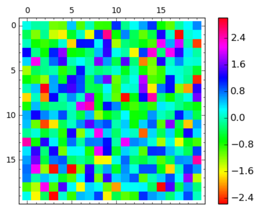
Fig. 89 A plot of a matrix of normally distributed numbers with a colorbar.

We have already a random coefficient matrix A. Let us generate a random right hand side vector b and solve a linear system A*x = b. The random numbers are uniformly distributed in the interval [-1,+1].

b = np.random.uniform(-1, 1, (20, 1))
x = np.linalg.solve(A, b)
v = b - A*x
r = np.linalg.norm(v)
r

What we see printed as the value of r is 18.1786344846. The residual r of a linear system is the norm of b - A*x, but something went wrong, because the residual is too large! What is the problem? Let us look at the type of A, b, and x.

print('type(A) :', type(A))
print('type(b) :', type(b))
print('type(x) :', type(x))

In all three cases, we see numpy.ndarray as the type. For the operator arithmetic to work properly, we must convert to the proper matrix types.

mA = np.matrix(A)
print(type(mA))
mb = np.matrix(b)
print(type(mb))
mx = np.matrix(x)
print(type(mx))

The variables mA, mb, and mx are instances of the class numpy.matrixlib.defmatrix.matrix. Now we can compute the residual correctly.

v = mb - mA*mx
r = np.linalg.norm(v)
r

As we see for the value of r the number 2.37857348102e-15 we see that the solution x of the linear system A*x = b is accurate within the machine precision for hardware doubles.

The fundamental data type in a MATrix LABoratory is a matrix and numpy gives matrices to Python. Vectorization is a technique to formulate linear algebra operations with vector and matrix arithmetic. The arithmetic is performed on dedicated data structures by optimized and fine tuned libraries.

Numerical Integration

Many expressions do not have symbolic antiderivatives.

f = exp(sin(x))
a = integral(f, x, 0, 1)
a

Sage then returns integrate(e^sin(x), x, 0, 1). It would have been better to set the hold flag to True, as in integrate(e^sin(x), 0, 1, hold=True). Then with a.n() we can get a numerical approximation. Sometimes we may directly go for a numerical approximation and apply quadrature rules.

from scipy.integrate import quad
d = quad(f, 0, 1, full_output=1)
d

Not only is the numerical approximation returned, but also an estimate for the error and the number of function evaluations. The first two numbers in the output are (1.6318696084180513, 1.8117392124517587e-14, which respectively give the approximation of the integral and the estimated error on the approximation.

Rational Approximations

Often we use a combination of sympy and scipy. For example, the computation of a Padé approximation starts from a Taylor series. We can compute Taylor series with sympy and Padé approximations with scipy.

from sympy import var, sin, series
x = var('x')
s = series(sin(x), x, 0, n=None)
terms = [next(s) for _ in range(6)]
terms

To extract the coefficients of the terms, we do

c = [sterms.coeff(x, k) for k in range(6)]
c

The coefficients of the series are [0, 1, 0, -1/6, 0, 1/120]. We import the pade command from scipy.misc. The first argument of pade is the list with the coefficients of the Taylor series. The second argument is the degree of the denominator of the rational approximation. So if we want a denominator of degree 2, we proceed as follows.

from scipy.interpolate import pade
p = pade(c, 2)
p

On return we get numpy polynomials, which have a nice string representation.

print(type(p[0]))
print('numerator :\n', p[0])
print('denominator :\n', p[1])

Starting from a Taylor series of order So the rational approximation is (-0.1167*x^3 + x)/(0.05*x^2 + 1).

The numpy polynomials are callable, so plotting is no problem and we compare with the plot of the actual sin(x) function.

sp = plot(sin(x), (x, -pi, pi), color='red')
pp = plot(p[0](x)/p[1](x), (x, -pi, pi))
(sp+pp).show()

The plot is displayed in Fig. 90.

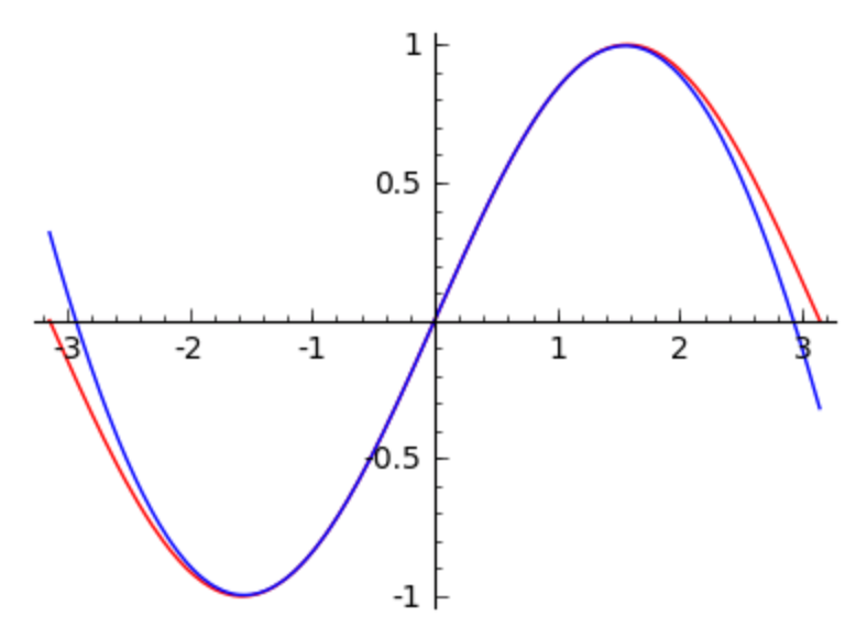
Fig. 90 A [3,2]-Padé approximation for the \(\sin(x)\) function.

The differences between the rational approximation and the sine function become noticeable only when x is less than -pi/2 or larger than pi/2.

We can use the function to bring the polynomials from scipy into SageMath objects.

fp0 = p[0](x)
print(fp0)
print(type(fp0))
sfp0 = SR(fp0)
print(sfp0, 'has type', type(sfp0))

The type of the expression is in this way converted by SR() from sympy.core.mul.Mul to a symbolic Sage expression.

Numerical Solving of Ordinary Differential Equations

We end with the numerical solving of an ordinary differential equation, taking the pendulum problem:

\[\frac{d^2 \theta}{d t^2} = -\frac{d \theta}{d t} - 9.8 \sin(\theta)\]

We need to define a system of first-order differential equations, introducing an extra variable velocity which is the derivative of theta. Denote \(v(t) = \frac{d \theta}{d t}\), then the second order ordinary differential equation becomes a system of two first order ordinary differential equations.

\[\begin{split}\left\{ \begin{array}{rcl} {\displaystyle \frac{d \theta}{d t}} & = & v \\ % \vspace{-1mm} \\ \\ {\displaystyle \frac{d v}{d t}} & = & {\displaystyle -\frac{d \theta}{d t} - 9.8 \sin(\theta).} \\ \end{array} \right.\end{split}\]

We could define the right hand side of the system as below.

t, theta, velocity = var('t, theta, velocity')
oderhs = [velocity, -velocity-9.8*sin(theta)]
oderhs

The right hand side of the system has to be defined as a function.

def pend(y, t):
    return [y[1], -y[1]-9.8*sin(y[0])]

The symbolic evaluation of this function returns the same as the oderhs from above. Then we import odeint of the scipy.integrate package.

from scipy.integrate import odeint
from scipy import linspace
npts = 1000 # number of points
tspan = linspace(0, 10, npts)
sol = odeint(pend, [pi/10, 0], tspan)
points = [(tspan[k], sol[k][0]) for k in range(npts)]
list_plot(points, size=1)

The outcome of list_plot() is shown in Fig. 91.

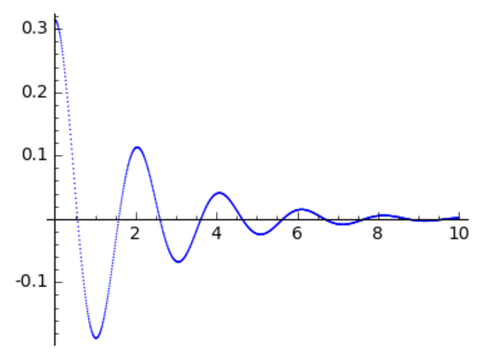
Fig. 91 The evolution of the displacement angle of the pendulum over time.

A phase portrait shows the displacements and the velocities. With a list comprehension we define the coordinates for the list plot.

coords = [(sol[k][0], sol[k][1]) for k in range(npts)]
list_plot(coords, size=1, figsize=4)

The phase portrait is shown in Fig. 92. The spiral shown in this figure should be interpreted as an inward moving spiral, as the pendulum comes to a halt. We see that the rightmost point corresponds to the point with coordinates \((\pi/10, 0)\) which matches the initial displacement angle and the initial velocity. As the trajectory spirals first down, the velocity vector is negative and we move towards the origin. At the leftmost end, we already notice the effect of the damping as the leftmost point is closer to the origin than the rightmost point.

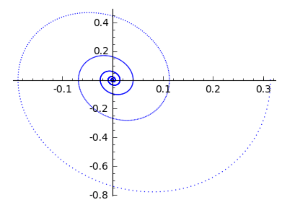
Fig. 92 The phase portrait of a damped pendulum.

Assignments

1. Define upper triangular matrices A that have ones on the diagonal and above the diagonal, for dimensions 2, 4, 8, 16, etc… The corresponding right hand side vector b is a vector of ones. Solve the linear systems A*x = b and report the residual, doubling the dimension in each case. How high can the dimension be before the residual becomes larger than 1.0e-8?

2. Let the \(n\)-dimensional matrix \(A\), where the \((i,j)\)-th element is defined as \(i^2 + j^2\), for \(i\) and \(j\) both ranging from 1 to \(n\). Do the following with numpy:

   1. Define \(A\) as a numpy matrix, for \(n = 17\).

      Define \({\bf b}\) as a 17-dimensional vector of ones.

   2. Solve the linear system \(A x = {\bf b}\) with numpy. Verify the residual.

      What is the sum of the coordinates in the solution \({\bf x}\)?

3. Use numpy to do the following.

   Define a tridiagonal 5-by-5 numpy matrix A: 3 on the diagonal and 1 just below and 1 just above the diagonal. Do NOT type in the 25 elements of A. Printing A shows:

   [[3 1 0 0 0]
    [1 3 1 0 0]
    [0 1 3 1 0]
    [0 0 1 3 1]
    [0 0 0 1 3]]
   

   Take as right hand side b a vector of all ones.

   Solve the system A*x = b and write the norm of the residual b - A*x.

4. Consider the function f(x) = exp(-x^2)*sin(2*k*pi*x) for increasing values of k, where k is 2, 4, 8, 16, 32, 64. Apply quad of scipy to approximate the integral of f(x) over the interval [-2, +2]. Report the number of function evaluations as k increases.

5. Compute a rational Padé approximation for cos(x), based on a Taylor series of order 6. Make a plot to compare the accuracy between the rational approximation and the cos(x).

6. Compute a rational Padé approximation for \(\tan(x)\), following the steps below.

   1. Generate a Taylor series of \(\tan(x)\) at \(x = 0\) order 6. Compute its list of coefficients.

   2. Use the coefficients to compute a Padé approximation where the denominator has degree 2. Write the rational expression you obtain.

   3. What is the difference between the value of \(\tan(\pi/4)\) and the approximation at \(\pi/4\)?

7. Consider the following system of differential equations:

   \[\begin{split}\left\{ \begin{array}{rcrcr} {\displaystyle \frac{d }{d t} r(t) } & = & 1.1 ~r(t) & - & 0.5 ~r(t) f(t) \\ % \vspace{-1mm} \\ {\displaystyle \frac{d }{d t} f(t) } & = & -0.75 ~f(t) & + & 0.25 ~r(t) f(t) \\ \end{array} \right. \quad \quad r(0) = 3, f(0) = 2.\end{split}\]

   This system can be used to model the evolution in time \(t\) of two species, with \(f(t)\) the size of the predator population (\(f\) = fox) and \(r(t)\) the size of the prey population (\(r\) = rabbit).

   1. Define the right hand side vector in a function for use in odeint to solve the system, with the time span for \(t\) going from 0 to 8.

   2. With these two functions, make a plot of the solution trajectories, for \(t\) going from 0 to 8.

   3. Use the numerical solutions to a phase portrait.