Lecture 43: Statistical Computing with R
R is a language and environment for statistical computing and graphics. We can run R from a terminal session or evaluate cells in a Sage notebook interface with R.
Computations with R
The R in Sage is a little r.
c = r('choose(5,2)')
print(c, 'has type', type(c))
print(c.sage())
With the sage() we convert an RElement into a corresponding
Sage expression.
We can evaluate R commands given as strings to r.eval().
The result of this evaluation is a string.
r.eval('choose(100, 30)')
Notice that ‘[1] 2.937234e+25’ contains a floating-point number. R is not a computer algebra package, unlike Sage. In Sage we compute binomials as follows.
print(binomial(5,2))
print(binomial(100,30))
To estimate \(\pi\) we can run a Monte Carlo simulation. We can use that
to estimate \(\pi\). We generate one million uniformly distributed points in the interval [0,1] and compute the mean of the height of the points.
data = r('u <- runif(1000000,min=0,max=1)')
estpi = r('4*mean(sqrt(1 - u^2))')
estpi
We see the estimate 3.142004.
To check, we use integrate.
f = r('integrand <- function(x) { sqrt(1-x^2) }')
i = r('integrate(integrand, lower=0, upper=1)')
i
The output is 0.7853983 with absolute error < 0.00011.
Plotting Data
We generate 100 random normally distributed numbers, sort the numbers, and then make a stem and leaf plot.
r.eval('rn = rnorm(100)')
print r.eval('sort(rn)')
p = r.eval('stem(rn)')
p
The stem and leaf plot is stored as a string in p.
The decimal point is at the |

-3 | 4
-2 | 72
-1 | 9665544332100
-0 | 999888877776665555444433333332222110
 0 | 001111222222333334455566667788999
 1 | 000224455569
 2 | 036
We illustrate the r.call() and making a histogram of data.
r.quartz() # to plot on Mac OS X
data = r.call('rnorm', 100)
r.call('hist', data)
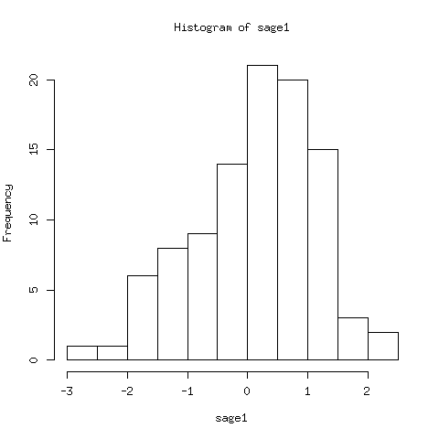
The data for the histogram is below. The histogram plot is in Fig. 98.
$breaks
[1] -3.0 -2.5 -2.0 -1.5 -1.0 -0.5  0.0  0.5  1.0  1.5  2.0  2.5
$counts
[1]  1  1  6  8  9 14 21 20 15  3  2
$density
[1] 0.02 0.02 0.12 0.16 0.18 0.28 0.42 0.40 0.30 0.06 0.04
$mids
[1] -2.75 -2.25 -1.75 -1.25 -0.75 -0.25  0.25  0.75  1.25  1.75  2.25

Fig. 98 A histogram of 100 random, normally distributed, data points.
Making a box plot of the data is straightforward.
r.call('boxplot', data)
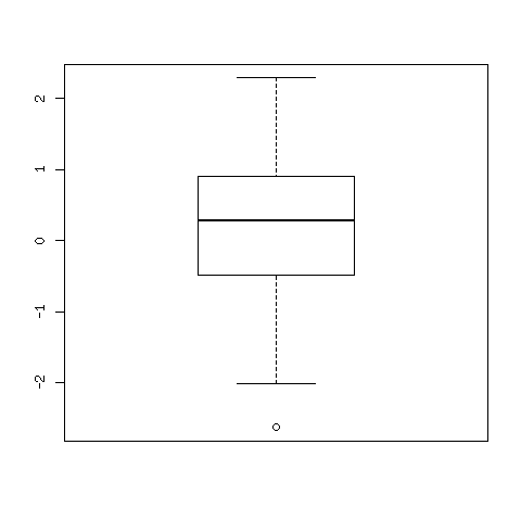
The data is shown below and the plot is in Fig. 99.
$stats
           [,1]
[1,] -2.0077439
[2,] -0.4777200
[3,]  0.2852553
[4,]  0.9061189
[5,]  2.2852012
$n
[1] 100
$conf
           [,1]
[1,] 0.06660879
[2,] 0.50390188
$out
[1] -2.620645

Fig. 99 A box plot of 100 random, normally distributed, data points.
The middle line in the plot indicates the medium. What is in the box are the points between the first and third quartile of the data. The horizontal lines at bottom and top show respectively the minimum and maximum of the data. Outliers are marked by circles.
Fitting Linear Models
To fit linear models, we apply lm.
As a test we generate 50 points in [0, 10] as x.
We set y equal to x with some random noise added.
Observe the assignment in r.
r('x <- 10*runif(50)')
r('y <- x + rnorm(50)')
r.quartz()
r('plot(x,y)')
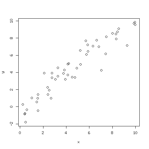
The plot is shown in Fig. 100.

Fig. 100 A plot of 50 points on a line with random noise added.
Now we do the fit with the command lm.
r('fit <- lm(y ~ x)')
For the output we can read off the intercept b and the slope a
for the linear fit y = a*x + b. See below:
Call:
lm(formula = y ~ x)

Coefficients:
(Intercept)            x
     0.1891       0.9573
We can ask for a summary.
r('summary(fit)')
The summary of the fit is below.
Call:
lm(formula = y ~ x)

Residuals:
     Min       1Q   Median       3Q      Max
-1.84906 -0.75229 -0.07965  0.40908  2.46077

Coefficients:
            Estimate Std. Error t value Pr(>|t|)
(Intercept)  0.18907    0.28316   0.668    0.508
x            0.95734    0.04729  20.245   <2e-16 ***
---
Signif. codes:  0 ‘***’ 0.001 ‘**’ 0.01 ‘*’ 0.05 ‘.’ 0.1 ‘ ’ 1

Residual standard error: 1.014 on 48 degrees of freedom
Multiple R-squared:  0.8952, Adjusted R-squared:  0.893
F-statistic: 409.8 on 1 and 48 DF,  p-value: < 2.2e-16