
Assignment One
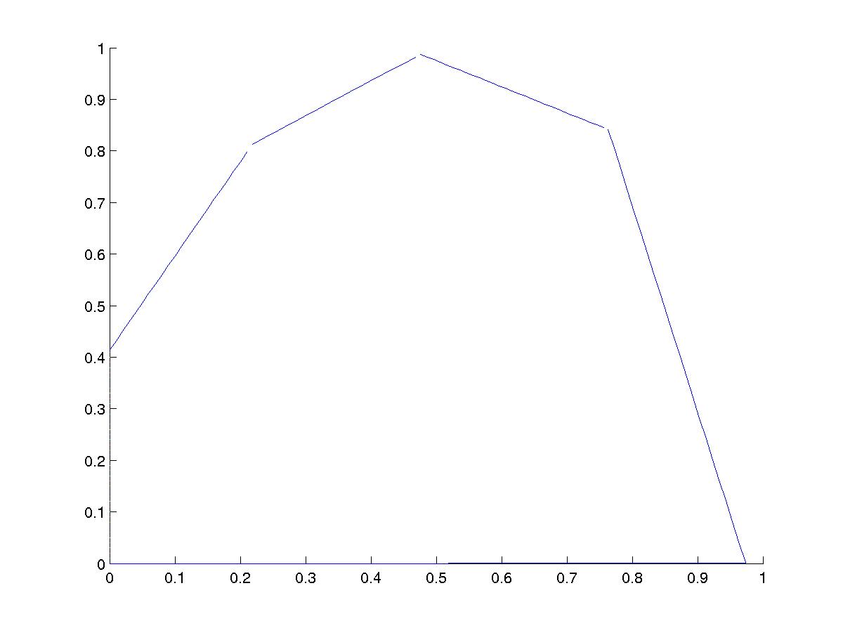
The number of steps of the simplex algorithm ranges between 2 and 4, with an average of about 3, obtained by 10 runs with random f values. If f(1) > f(2), the path of vertices visited by the algorithm will start turning right and move counterclockwise to the optimal solution; otherwise it will start going upwards and move clockwise to the optimum. Drawing the objective function through the optimal solution, we see the ordering of the vertex points.
Here are the data produced by the first script (see appendix):
sA =

    0.7499   -1.0000
    0.8930    0.3784
    0.4126    0.8141
   -0.6756    1.0000
   -1.0000    0.5473


sb =

    0.3850
    1.0000
    1.0000
    0.6654
    0.2264


n =

     2
     3
     3
     3
     3
     3
     4
     3
     3
     3


ans =

     3
Assignment Two
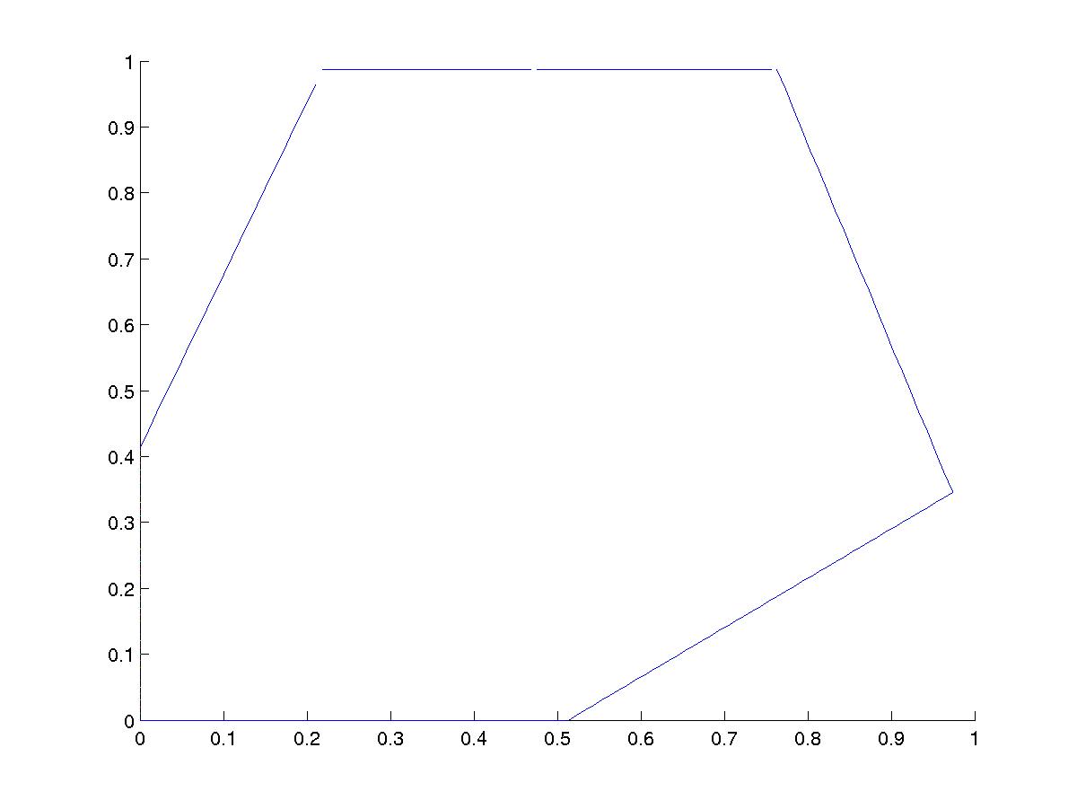
We get high numbers in an intermediate tableau when we take the vertex with the highest x(1)-coordinate very close to the x-axis. This vertex will be the optimal solution if we take f(2) = 0. The value of x(2) of the optimal solution is 1.0e-8.
When the simplex algorithm hops from (0,0) to the first vertex at the right with coordinates (a,0), we see values of order 1.0e+7 appearing after the diagonalization. Note that for this run we modified the simplex algorithm, adding one line with "t" on it after the diagonalize() to see the tableau after pivoting. At the vertex where these high numbers occur, we have two edges which are almost parallel to each other. This is an ill-conditioned vertex.
Notice that this behaviour depends on the tolerance, when 1.0e-9 is taken as the value for x(2) of the optimal solution, then we do not see such high numbers.
To improve the numerical stability in the case where we saw the huge numbers, we should use a higher tolerance, say 1.0e-6 instead of 1.0e-8. If the tolerance is 1.0e-6, then pivots of size smaller than 1.0e-6 will not be taken.
Here is the data produced by the second script (see appendix):
sA =

    0.0000   -1.0000
    1.0000    0.2500
    0.4126    0.8141
   -0.6756    1.0000
   -1.0000    0.5473


sb =

    0.0000
    0.9736
    1.0000
    0.6654
    0.2264


t =

   1.0e+07 *

  Columns 1 through 6

         0    4.6020   -4.6020         0         0         0
    0.0000   -4.6020    4.6020         0         0         0
         0    4.6020   -4.6020    0.0000         0         0
         0    1.8986   -1.8986         0    0.0000         0
         0   -3.1091    3.1091         0         0    0.0000
         0   -4.6020    4.6020         0         0         0

  Columns 7 through 8

         0   -0.0000
         0    0.0000
         0    0.0000
         0    0.0000
         0    0.0000
    0.0000    0.0000


t =

  Columns 1 through 6

         0         0   -0.2500   -1.0000         0         0
    1.0000         0    0.2500    1.0000         0         0
         0    1.0000   -1.0000    0.0000         0         0
         0         0    0.7109   -0.4126    1.0000         0
         0         0    1.1689    0.6756         0    1.0000
         0         0    0.7973    1.0000         0         0

  Columns 7 through 8

         0   -0.9736
         0    0.9736
         0    0.0000
         0    0.5983
         0    1.3232
    1.0000    1.2000


inb =

     1     2     5     6     7


otb =

     3     4


x =

  Columns 1 through 6

    0.9736    0.0000         0         0    0.5983    1.3232

  Column 7

    1.2000


v =

    0.9736


n =

     2


t =

  Columns 1 through 6

         0   -0.2500         0   -1.0000         0         0
    0.0000   -1.0000    1.0000         0         0         0
    1.0000    0.2500         0    1.0000         0         0
         0    0.7109         0   -0.4126    1.0000         0
         0    1.1689         0    0.6756         0    1.0000
         0    0.7973         0    1.0000         0         0

  Columns 7 through 8

         0   -0.9736
         0    0.0000
         0    0.9736
         0    0.5983
         0    1.3232
    1.0000    1.2000


inb =

     3     1     5     6     7


otb =

     4     2


x =

  Columns 1 through 6

    0.9736         0    0.0000         0    0.5983    1.3232

  Column 7

    1.2000


v =

    0.9736


n =

     1
Assignment Three
To make the optimal solution ill-conditioned, we need it to be the
intersection of two edges which run almost parallel to each other.
For example, we elevated the two vertices adjacent to the vertex
with the highest value of x(2), using the value x(2) - 1.0e-7 for
their new x(2) coordinates. The vertex with the highest x(2) value
becomes optimal with f = [0 1]. Its two adjacent vertices have
a value of the objective function which differs by only 1.0e-7.
The condition of the defining linear equations at this vertex
is 1.0e+6.
With a condition number of 10^6, we can lose up to 6 decimal places accuracy in our final answer. As the difference in height between the optimal vertex and its two adjacent neighbors is 10^(-7), we can afford condition numbers up to 10^9. If the condition number would pass 10^9, we can no longer be sure of reaching the correct vertex. In this case, any point on the top edge is a likely solution.
We could remedy the numerical conditioning by a sensitivity analysis: just look at the vertices adjacent to the optimal solution. In this case, we have actually almost an entire edge which is optimal, there are close to having infinitely many solutions.
Here is the data produced by the third script (see appendix):
sA =

    0.7499   -1.0000
    0.9202    0.3016
    0.0000    1.0000
   -0.0000    1.0000
   -1.0000    0.3813


sb =

    0.3850
    1.0000
    0.9871
    0.9871
    0.1577


ans =

   2.7144e+06
Appendix: scripts for the three assignments.
The data in the tables above is produced by running three scripts, using three auxiliary functions: septagon, plotgon, and scale.
the function septagon
function [A,b] = septagon(v)
%
%  returns the system of linear inequalities defining a septagon,
%  of the type A*x <= b
%
%  on entry:
%    v         7-by-2 matrix, columns are x and y-coordinates:
%                v(:,1) = x and v(:,2) = y
%
%  on return:
%    A         7-by-2 matrix with coefficients of linear inequalities;
%    b         constant coefficients of the linear inequalities.
%
%  required:
%    the vertices are ordered counterclockwise, starting at (0,0).
%
x = v(:,1);     y = v(:,2);
n = length(x);
A = zeros(7,2); b = zeros(7,1);
for i=1:n
  if(i+1 > n)
    i1 = 1;
  else
    i1 = i+1;
  end;
  dx = x(i1) - x(i);  A(i,2) = -dx;
  dy = y(i1) - y(i);  A(i,1) = dy;
  b(i) = dy*x(i) - dx*y(i);
  if (b(i) < 0)
    b(i) = -b(i);  A(i,:) = -A(i,:);
  end;
end;
the function plotgon.m
function plotgon(v,A,b)
%
%  makes a plot of the polygon with vertices in v
%
%  on entry:
%    v         7-by-2 matrix, columns are x and y-coordinates:
%                v(:,1) = x and v(:,2) = y
%    A         coefficients of the linear inequalities;
%    b         right hand side vector of the system A*x <= b.
%
%  required:
%    the vertices are ordered counterclockwise, starting at (0,0).
%
figure;
hold on
x = v(:,1); y = v(:,2);
n = length(x);
r = 0.01;
for i=1:n
  if(i+1 > n)
    i1 = 1;
  else
    i1 = i+1;
  end;
  if (x(i) < x(i1))
    xr = x(i):r:x(i1);
  else
    xr = x(i1):r:x(i);
  end;
  if (A(i,2) ~= 0.0)
    yr = (b(i) - A(i,1)*xr)/A(i,2);
  else
    if (y(i) < y(i1))
      yr = y(i):r:y(i1);
    else
      yr = y(i1):r:y(i);
    end;
  end;
  plot(xr,yr);
end;
the function scale.m
function [A,b] = scale(A,b)
%
%  scales the inequalities so that the largest coefficient in
%  every inequality equals one
%
%  on entry:
%    A         7-by-2 matrix with coefficients of linear inequalities;
%    b         constant coefficients of the linear inequalities.
%
n = length(b);
for i=1:n
  m = max(abs([A(i,:) b(i)]));
  A(i,:) = A(i,:)/m;
  b(i) = b(i)/m;
end;
Script for Assignment One
diary output_one.txt;
v = [ .0000   .0000;
      .5134   .0000;
      .9736   .3451;
      .7632   .8416;
      .4761   .9871;
      .2187   .8132;
      .0000   .4136  ]
[A,b] = septagon(v)
[A,b] = scale(A,b)
plotgon(v,A,b);
sA = A(2:6,:)
sb = b(2:6)
tol = 1.0e-8;
n = zeros(10,1);
for i=1:10
  f = rand(2,1);
  [t,inb,otb,x,v,n(i,1)] = simplex(f,sA,sb,tol);
end;
n
sum(n)/10
xr = x(1)-0.1:0.01:x(1)+0.1;
yr = x(2) - f(1)/f(2)*(xr - x(1));
plot(xr,yr,'r');
diary off;
Script for Assignment Two
diary output_two.txt;
v = [ .0000   .0000;
      .5134   .0000;
      .9736   1.0e-8;
      .7632   .8416;
      .4761   .9871;
      .2187   .8132;
      .0000   .4136  ];
[A,b] = septagon(v);
[A,b] = scale(A,b);
plotgon(v,A,b);
sA = A(2:6,:)
sb = b(2:6)
tol = 1.0e-8;
f = [1 0];
[t,inb,otb,x,v,n] = simplex(f,sA,sb,tol)
tol = 1.0e-6;
[t,inb,otb,x,v,n] = simplex(f,sA,sb,tol)
diary off;
Script for Assignment Three
diary output_three.txt;
v = [ .0000   .0000;
      .5134   .0000;
      .9736   .3451;
      .7632   .9871 - 1.0e-7;
      .4761   .9871;
      .2187   .9871 - 1.0e-7;
      .0000   .4136  ];
[A,b] = septagon(v);
[A,b] = scale(A,b);
plotgon(v,A,b);
sA = A(2:6,:)
sb = b(2:6)
tol = 1.0e-8;
f = [0 1];
[t,inb,otb,x,v,n] = simplex(f,sA,sb,tol);
cond([sA(3,:); sA(4,:)])
diary off;