Systems of Ordinary Differential Equations¶

In this lecture, we continue our study of differential equations to model various problems, to arrive at traffic, a rich source of problems. We end with nonlinear systems.

Models of Pursuit¶

We start with the tractrix problem as a model of pursuit. Consider a trailer attached to a tractor. For example: a toddler pulling the string attached to a toy car.

Input: $(x_1(t), x_2(t))$ is the path of the tractor.
Output: $(y_1(t), y_2(t))$ is the path of the trailer.

The coordinate functions $y_1(t)$ and $y_2(t)$ are the solutions of a system of two ordinary differential equations.

To derive the differential equations, consider the following. The velocity vector of the trailer is parallel to the direction of the bar that connects trailer to tractor:

\[\begin{split}\left( \begin{array}{c} y_1' \\ y_2' \end{array} \right) = \lambda \left( \begin{array}{c} x_1 - y_1 \\ x_2 - y_2 \end{array} \right), \quad \lambda > 0.\end{split}\]

Observe:

$(y_1'(t), y_2'(t))$ is the change in position of the trailer.
$(x_1(t) - y_1(t), x_2(t) - y_1(t))$ is the direction vector.

The velocity vector of the trailer is the projection of the direction vector of the trailer onto the direction of the bar:

\[u = \frac{(x_1 - y_1 , x_2 - y_2)}{||(x_1 - y_1 , x_2 - y_2)||} \quad {\rm and} \quad v = (x_1', x_2'),\]

we compute the projection of the velocity vector as $(v^T u) u$. Then the system of first-order equations that defines the path of the trailer is given by

\[\begin{split}\left( \begin{array}{c} y_1' \\ y_2' \end{array} \right) = (v^T u) u,\end{split}\]

where

$u$ is the normalized vector of the direction of the bar, and
$v$ is the velocity vector of the tractor.

In the simulation, we assume a simple path of the tractor. The tractor moves on a circle, counter clockwise, as defined in the function below:

"""
    function tractor(time::Float64)

returns a 4-tuple xp, yp, xv, yv, with
the coordinates xp, yp of the position, and
the components xv, yv of the velocity vector
for the tractor at the given time.
"""
function tractor(time::Float64)
    xpos = cos(time)
    ypos = sin(time)
    xvel = -sin(time)
    yvel = cos(time)
    return (xpos, ypos, xvel, yvel)
end

The right hand side of the system of ordinary differential equations is defined by the function below:

"""
    function trailer!(du::Vector{Float64},
                      u::Vector{Float64}, p, t)

defines the right hand side of the system.
"""
function trailer!(du::Vector{Float64},
                  u::Vector{Float64}, p, t)
    x1p, x2p, x1v, x2v = tractor(t)
    du[1] = x1p - u[1]
    du[2] = x2p - u[2]
    nrm = sqrt(du[1]*du[1] + du[2]*du[2])
    du[1] = du[1]/nrm
    du[2] = du[2]/nrm
    vtu = x1v*du[1] + x2v*du[2]
    du[1] = vtu*du[1]
    du[2] = vtu*du[2]
end

The code to solve and plot follows:

timespan = (0, 20)

initconds = [2.0, 0.0]

odetractrix = ODEProblem(trailer!, initconds, timespan)

soltractrix = solve(odetractrix)

trailerpath = [(x,y) for (x,y) in soltractrix.u]

runcircle = [tractor(t) for t=0:0.01:2*pi]
tractorpath = [(tpl[1],tpl[2]) for tpl in runcircle]

plot(tractorpath, label="tractor")
plot!(trailerpath, label="trailer")

The solution trajectory is shown in Fig. 94.

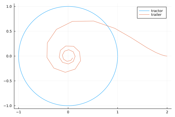
_images/figTractorTrailer.png — Fig. 94 The trajectories of a trailer and a tractor.¶

With saveat=0.05 we obtain a smoother plot, shown in Fig. 95.

_images/figTractorTrailer2.png — Fig. 95 A smooth plot of the trajectory of the trailer.¶

Code to define an animation is below:

animTractorTrailer = Plots.Animation()
for i = 10:10:length(tractorpath2)
    plot(tractorpath2[1:i], label="tractor",
         xlims=(-1.1,2.1), ylims = (-1.1, 1.1))
    (xtp1, xtp2) = tractorpath2[i]
    scatter!([xtp1], [xtp2], legend=false)
    plot!(trailerpath2[1:i], label="trailer")
    Plots.frame(animTractorTrailer)
end

gif(animTractorTrailer, "tractortrailer2.gif", fps = 2)

Related to the tractrix problem is that of a predator chasing a prey, the predator-prey problem:

Input: $(x_1(t), x_2(t))$ is the path of the prey.
Output: $(y_1(t), y_2(t))$ is the path of the predator.

The velocity vector of the predator is parallel to the direction of predator towards the prey:

\[\begin{split}\left( \begin{array}{c} y_1' \\ y_2' \end{array} \right) = \lambda \left( \begin{array}{c} x_1 - y_1 \\ x_2 - y_2 \end{array} \right), \quad \lambda > 0.\end{split}\]

Observe:

$(y_1'(t), y_2'(t))$ is the change in position of the prey
$(x_1(t) - y_1(t), x_2(t) - y_1(t))$ is the direction vector.

As in the tractrix model, the velocity vector of the predator is the projection of the direction vector of the predator towards the prey:

\[\begin{split}\left( \begin{array}{c} y_1' \\ y_2' \end{array} \right) = s(t)~\!u,\end{split}\]

with

\[u = \frac{(y_1 - x_1 , y_2 - x_2)}{||(y_1 - x_1 , y_2 - x_2)||}\]

where $s(t)$ is the speed of the predator, for example:

$s(t) = c$, at constant speed $c$, or
$s(t) = a~\!t$, with acceleration $a$.

As before, in the tractrix problem, the predator moves in a circle (calling the function tractor), but with accelerating speed, as defined below:

"""
    function predator!(du::Vector{Float64},
                       u::Vector{Float64}, p, t)

defines the right hand side of the system for the
predator, chasing a prey with accelerating speed.
"""
function predator!(du::Vector{Float64},
                   u::Vector{Float64}, p, t)
    x1p, x2p, x1v, x2v = tractor(t)
    acceleration = p
    speed = acceleration*t
    du[1] = x1p - u[1]
    du[2] = x2p - u[2]
    nrm = sqrt(du[1]*du[1] + du[2]*du[2])
    du[1] = speed*du[1]/nrm
    du[2] = speed*du[2]/nrm
end

The trajectory of a predator in pursuit of a prey, with acceleration = 0.1 is shown in Fig. 96.

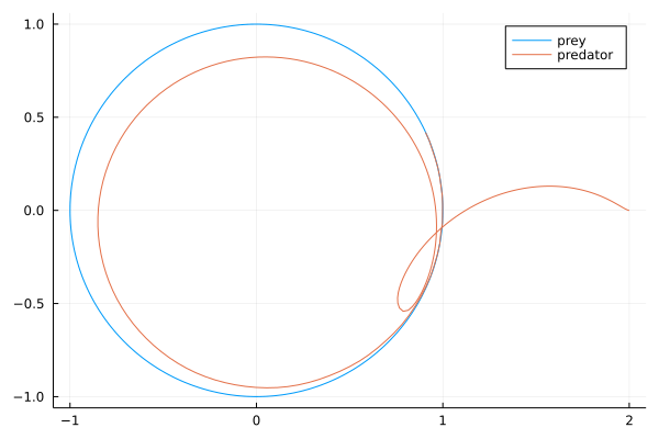
_images/figPredatorPrey1.png — Fig. 96 The trajectory of a prey chased by a predator.¶

The interpretation of Fig. 96 benefits from an animation.

The speed of the predator is $s(t) = 0.1 t$.

For small $t$, the speed $0.1 t$ is very small, and the predator moves very slowly.
Once $t$ goes past 10, the speed of the predator becomes larger than one.
The prey remains circling at unit speed. So eventually, the predator catches the prey.

Multiple Mass Springs and Traffic¶

Consider a mass $m$ sliding along a frictionless horizontal table, restrained by a spring, shown in Fig. 97. The displacement from equilibrium is $x(t)$.

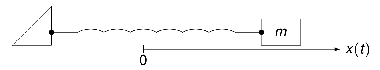
_images/figOneSpringMass.png — Fig. 97 One mass sliding along a frictionless table connected to a spring.¶

By Newton’s law, the inertial force is $\displaystyle m \frac{d^2}{d~\!t} x(t)$. The restoring force of the spring is proportional to $x(t)$, so we obtain

\[m \frac{d^2}{d~\!t} x(t) + k x(t) = 0, \quad \mbox{for some constants } k.\]

Three masses $m_1$, $m_2$, $m_3$, connected by springs are shown in Fig. 98.

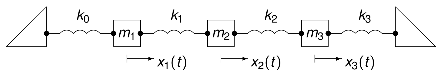
_images/figMultiSpringMass.png — Fig. 98 Three masses connected by springs.¶

The second mass receives a push

from $m_1$ with spring constant $k_1$, and
from $m_3$ with spring constant $k_2$,

compensated by the sum of $k_1$ and $k_2$:

\[m_2 \frac{d^2}{d~\!t^2} x_2(t) = k_1 x_1(t) - (k_1+k_2) x_2 + k_2 x_3(t).\]

The multiple mass spring system is then

\[m_1 x''_1(t) = \hphantom{k_1 x_1(t)} - (k_0+k_1) x_1 + k_1 x_2(t),\]

\[m_1 x''_2(t) = k_1 x_1(t) - (k_1+k_2) x_2 + k_2 x_3(t),\]

\[m_1 x''_3(t) = k_2 x_2(t) - (k_2+k_3) x_3 \hphantom{~+ k_2 x_3(t)}.\]

The multiple masses connected by springs inspired a car following theory. Consider a platoon of cars:

$x_1(t)$ is the position of the first vehicle at time $t$,
$x_k(t)$ is the position of the k-th vehicle in the platoon.

What happens in reaction to a disturbance? A model for the change in velocity caused by a difference in the velocity of the previous vehicle is

\[x_k''(t + \Delta t) = \alpha \left( \vphantom{\frac{1}{2}} x'_{k-1}(t) - x'_k(t) \right), \quad \mbox{for } k > 1,\]

where

$\Delta t$ is the reaction time of the $k$-th driver,
$\alpha$ is a sensitivity parameter.

Empirical values: $\Delta t \approx 1.55 \mbox{~sec}$ and $\alpha \approx 0.37 \mbox{~sec}^{-1}$.

Distance equals speed multiplied with the time traveled.

\[\begin{split}\begin{array}{rcl} d_k(t) & = & x_{k-1}(t) - x_k(t) \\ & = & {\displaystyle \int_0^t \left( \vphantom{\frac{1}{2}} x'_{k-1}(s) - x'_k(s) \right) ds + d}, \end{array}\end{split}\]

where $d$ is the initial distance between the vehicles. Use

\[x_k''(t + \Delta t) ~=~ \alpha \left( \vphantom{\frac{1}{2}} x'_{k-1}(t) - x'_k(t) \right)\]

to obtain

\[\begin{split}\begin{array}{rcl} d_k(t) & = & {\displaystyle \int_0^t \frac{x''_k(s + \Delta t)}{\alpha} ds + d} \\ & = & {\displaystyle \frac{1}{\alpha} \left( \vphantom{\frac{1}{2}} v_k(t+\Delta t) - v_k (0 + \Delta t) \right) + d} \\ & = & {\displaystyle \frac{1}{\alpha} v_k(t + \Delta t) - \frac{v}{\alpha} + d}, \end{array}\end{split}\]

where $v \approx v(\Delta t)$, when $\Delta t$ is small enough. Deriving an upper limit on the speed to avoid a collision:

\[-\frac{v}{\alpha} + d > 0 \quad \Rightarrow \quad v < \alpha d \quad \mbox{or} \quad d > v/\alpha.\]

Observe:

$v < \alpha d$ is an upper limit on the speed, or
$d > v/\alpha$ is a lower bound on the distance.

$\alpha \approx 0.37\mbox{~sec}^{-1}$, $1/\alpha \approx 2.7 \mbox{~sec}$, which gives rise to the 3 second rule.

We derived $d > v/\alpha$ as a lower bound on the distance to avoid a collision. The empirical values

\[\alpha \approx 0.37\mbox{~sec}^{-1} \quad \mbox{and} \quad 1/\alpha \approx 2.7 \mbox{~sec},\]

give rise to the 3 second rule, as $d > 2.7 v$.

The distance between two vehicles should be larger than the distance traveled in three seconds.

For information on Defensive Driving Courses, see the publication of the National Safety Council, 2019, on The DDC Instructor And Administrative Reference Guide.

Nonlinear Systems¶

To introduce the first nonlinear system, consider the problem of administering half a pill a day. The administering happens as follows. In taking a pill from the bottle:

If it is a half pill, then we just take it.
If the pill is whole, then
- break the pill in half, keep one half,
- throw the other half in the bottle.

Here is then our question: After k days, how many whole pills are left in the bottle?

To derive the equation on the number of whole pills, we introduce some notations.

Let $x_k$ the expected number of whole pills, at day $k$.
Let $y_k$ the expected number of half pills, at day $k$.

Consider now day $k+1$:

\[x_{k+1} - x_k = - \frac{x_k}{x_k + y_k}\]

is the expected net change in whole pills, as the number will decrease only if whole pill is drawn.

The ratio $\displaystyle \frac{x_k}{x_k + y_k}$ is the ratio of the number of whole pills, over the total number of pills.

For half pills, we have the equation:

\[y_{k+1} - y_k = \frac{x_k}{x_k + y_k} - \frac{y_k}{x_k + y_k},\]

which is

the increase if a whole pill is drawn, and
the decrease if a half pill is drawn.

Next, we introduce expected percentages

\[p_k = \frac{x_k}{N} \quad \mbox{and} \quad q_k = \frac{y_k}{N}.\]

The equations on the expected number of whole and half pills

\[\begin{split}\begin{array}{rcl} x_{k+1} - x_k & = & {\displaystyle - \frac{x_k}{x_k + y_k}} \\ y_{k+1} - y_k & = & {\displaystyle \frac{x_k}{x_k + y_k} - \frac{y_k}{x_k + y_k}} \end{array}\end{split}\]

is then rewritten with $p_k = x_k/N$ and $q_k = y_k/N$ into

\[\begin{split}\begin{array}{rcl} {\displaystyle \frac{p_{k+1} - p_k}{1/N}} & = & {\displaystyle - \frac{p_k}{p_k + q_k}} \\ {\displaystyle \frac{q_{k+1} - q_k}{1/N}} & = & {\displaystyle \frac{p_k}{p_k + q_k} - \frac{q_k}{p_k + q_k}}. \end{array}\end{split}\]

The original discrete formulation has a continuous version:

\[\begin{split}\begin{array}{rcl} {\displaystyle \frac{d}{d~\!t}~\!p(t)} & = & {\displaystyle - \frac{p}{p + q}} \\ {\displaystyle \frac{d}{d~\!t}~\!q(t)} & = & {\displaystyle \frac{p}{p + q} - \frac{q}{p + q}} \end{array}\end{split}\]

with initial conditions $p(0) = 1$ and $q(0) = 0$. Note that the system is deterministic.

Consider a model for an arms race, which also starts from ratios and leads to a system. Two nations $X$ and $Y$ are competing in an arms race. At year $n$,

\[x_n = \frac{\mbox{arms expenditure of nation $X$}} {\mbox{gross national product of $X$}}\]

\[y_n = \frac{\mbox{arms expenditure of nation $Y$}} {\mbox{gross national product of $Y$}}\]

We have $0 < x_n, y_n < 1$.

Both nations are reacting to each other:

\[\begin{split}\left\{ \begin{array}{rcl} x_{n+1} & = & 4 a~\!y_n (1-y_n) \\ y_{n+1} & = & 4 b~\!x_n (1-x_n) \end{array} \right.\end{split}\]

for parameters $a, b \in [0,1]$.

This is a coupled nonlinear system of difference equations.

Looking for fixed points, we eliminate $y_n$:

\[\begin{split}\begin{array}{rcl} x_{n+2} & = & 4~\!a~\!y_{n+1} (1-y_{n+1}) \\ & = & 16~\!a~\!b~\! x_n(1-x_n)(1 - 4~\!b~\!x_n(1-x_n)) \end{array}\end{split}\]

At the fixed point:

\[x = 16 a~\!b~\! x(1-x)(1 - 4~\!b x(1-x)).\]

Dividing out the trivial solution $x=0$ leads a cubic.

Proposal for a Topic of a Project¶

Take data on expressway traffic. At various times of the day:

What is the separation between cars?
What is the separation versus velocity?
How is flow related to density?

When is the road most dangerous?

Exercises¶

Consider rabbits and foxes, respectively the preys and predators.
- Let $r(t)$ denote the population of the rabbits.
- Let $f(t)$ denote the population of the foxes.
The system that models their evolution is

\[\begin{split}\left\{ \begin{array}{rcl} {\displaystyle \frac{d}{d~\!t} r(t)} & = & a~\!r(t) - b~\!r(t)f(t), \\ \\ {\displaystyle \frac{d}{d~\!t} f(t)} & = & -c~\!f(t) + d~\!r(t)f(t). \\ \end{array} \right.\end{split}\]
1. Let $a = 1.1$, $b = 0.5$, $c = 0.75$, $d = 0.25$, $r(0) = 3$, and $f(0) = 2$.
  
  Set up the system of differential equations and solve it, for the time span $[0, 10]$.
2. Plot the trajectories for $r(t)$ and $f(t)$.
  
  What is the end value for $t$ for one complete orbit?
Consider the three masses connected by springs. Write the system of second order differential equations as a system of first order differential equations, in matrix format.
Consider

\[\begin{split}\begin{array}{rcl} {\displaystyle \frac{d}{d~\!t}~\!p(t)} & = & {\displaystyle - \frac{p}{p + q}} \\ {\displaystyle \frac{d}{d~\!t}~\!q(t)} & = & {\displaystyle \frac{p}{p + q} - \frac{q}{p + q}} \end{array}\end{split}\]

with initial conditions $p(0) = 1$ and $q(0) = 0$.

Solve the system. Interpret the solution.
An equation of degree three such as

\[1 = 16 a~\!b~\! (1-x)(1 - 4~\!b x(1-x))\]

has one or three real roots.

Consider the following values for $a$ and $b$:
1. $a = 0.8, b = 0.4$,
2. $a = 0.8, b = 0.86$,
3. $a = 0.8, b = 0.9$.
Answer the following questions:
1. How many real roots in each case?
2. For each case, make plots of $x_n$. Interpret the plots.

Systems of Ordinary Differential Equations¶

Models of Pursuit¶

Multiple Mass Springs and Traffic¶

Nonlinear Systems¶

Proposal for a Topic of a Project¶

Exercises¶

Table of Contents

Previous topic

Next topic

This Page