Traffic Flow Modeling

We derive the continuity equation to study traffic flow and explore the Greenshields model to relate flow, speed and concentration.

Counting Cars

On two measure points (e.g., one mile apart), we count cars, as shown in Fig. 138.

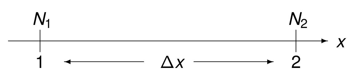
Fig. 138 Counting cars between two measure points.

In Fig. 138:

• \(N_1\) is the number of cars counted at point 1,

• \(N_2\) is the number of cars counted at point 2.

Denote \(\Delta N = N_2 - N_1\). The direction of traffic moves from 1 to 2. If \(\Delta N < 0\), then \(N_2 < N_1\), and there more cars at 1 than at 2, which means that the concentration of cars between 1 and 2 increases.

Let \(q\) be the number of cars per time unit \(\Delta t\).

\[\begin{split}\begin{array}{rcl} q_2 & = & N_2/\Delta t \\ - q_1 & = & N_1/\Delta t \\ \hline \Delta q & = & \Delta N/\Delta t \end{array}\end{split}\]

We have \(\Delta N = \Delta q \Delta t\). As \(\Delta t > 0\), \(\Delta q\) has the same sign as \(\Delta N\). If \(\Delta N < 0\), when the concentration of cars increases, then \(\Delta q < 0\) and the flow of cars decreases.

Let \(k\) be the number of cars per unit length \(\Delta x\).

\[\begin{split}\begin{array}{rcl} k_1 & = & N_1/\Delta x \\ - k_2 & = & N_2/\Delta x \\ \hline \Delta k & = & (-\Delta N)/\Delta x \end{array}\end{split}\]

If \(\Delta N < 0\), then the flow of cars decreases and the concentration increases, as \(\Delta N < 0\) implies \(\Delta k > 0\).

If there is no exit nor entry between the measure points 1 and 2, then we have continuity and

\[\begin{split}\begin{array}{rcl} \Delta N & = & \hphantom{-} \Delta q \Delta t, \\ \Delta N & = & - \Delta k \Delta x. \end{array}\end{split}\]

Eliminating \(\Delta N\) leads to \(\Delta q \Delta N = - \Delta k \Delta x\), or equivalently:

\[\frac{\Delta q}{\Delta x} + \frac{\Delta k}{\Delta t} = 0.\]

Taking limits as \(\Delta x \rightarrow 0\) and \(\Delta t \rightarrow 0\), we have the continuity equation

\[\frac{\partial q}{\partial x}(x, t) + \frac{\partial k}{\partial t}(x, t) = 0.\]

Adding the change in flow to the change in concentration equals zero.

Speed, Flow, and Concentration

We introduce the Greenshields model. Observe the units:

• The units of concentration \(k\) are the number of cars per mile.

• The units of speed \(v\) are the number of miles per hour.

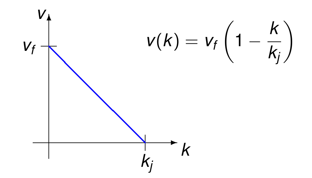
Fig. 139 Speed in function of concentration.

In the Greenshields model, as shown in Fig. 139, the speed depends on the concentration.

• \(v_f\) is the free traffic speed, when the road is free.

• \(k_j\) is the jam density, \(v=0\) at a traffic jam.

We can flip the axes in Fig. 139 and express concentration in function of speed:

\[\begin{split}v(k) = v_f \left( 1 - \frac{k}{k_j} \right) = v_f \left( \frac{k_j - k}{k_j} \right) \quad \Rightarrow \quad \begin{array}{l} k_j v = v_f ( k_j - k) \\ k_j v - v_f k_j = - k v_f \end{array}\end{split}\]

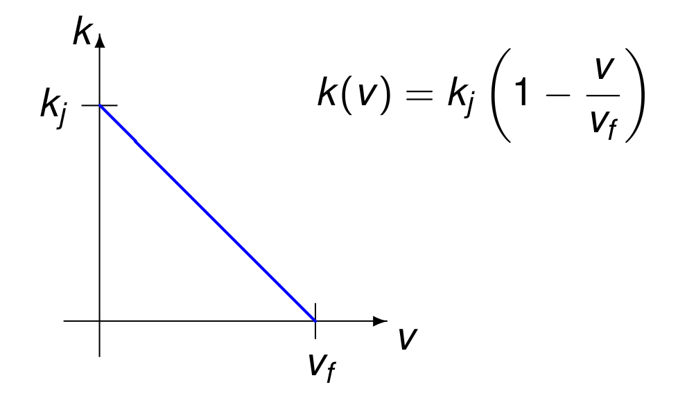
Fig. 140 Concentration in function of speed.

In the Greenshields model, as shown in Fig. 140, the concentration depends on the speed.

• If \(v = 0\), then traffic is jammed and \(k = k_j\).

• If \(v = v_f\), then there is no traffic and \(k = 0\).

While \(v_f\) can be set to the speed limit, the jam density \(k_j\) is the intercept of a least squares fit, as shown in Fig. 141.

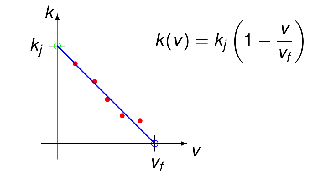
Fig. 141 The solid red dots represent observed data points.

Now let us express flow as a function of concentration. Speed \(v\) and concentration \(k\) are linearly correlated. Flow \(q\) is expressed in the number of cars per hour. Observe the following:

• If \(k = 0\) (no cars per mile), then no cars per hour, \(q = 0\).

• If \(k = k_j\) (traffic is jammed), then no speed and no flow either.

• The maximum flow occurs for some \(k\) in between zero and \(k_j\).

Flow and concentration can thus not be correlated linearly. Therefore, let us use a concave down parabola.

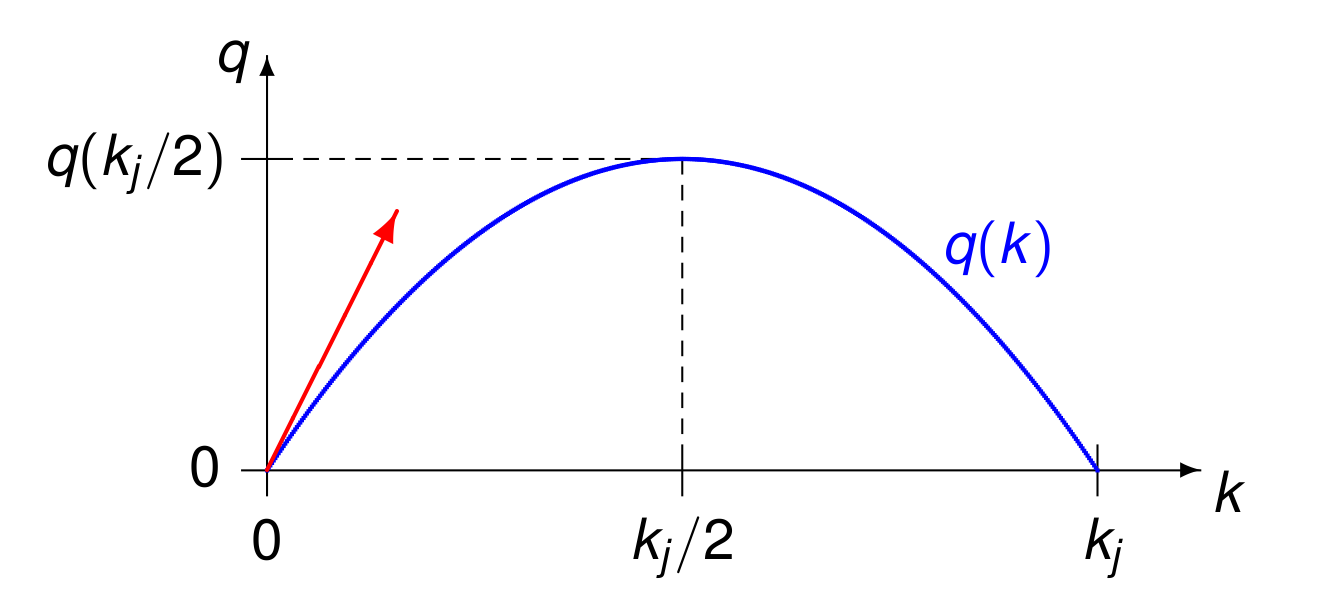
Fig. 142 Flow in function of concentration.

A parabolic model for flow, shown Fig. 142, as function of concentration is:

\[q(k) = a_2 k^2 + a_1 k + a_0\]

Observe the following:

1. \(q(0) = 0 \Rightarrow a_0 = 0\),

2. \(q'(k) = 2 a_2 k + a_1 \Rightarrow a_1 = q'(0)\),

3. \(q''(k) = 2 a_2 < 0\), concave down.

Where is \(v_f\)? Look at Fig. 142.

There is no flow at the traffic jam:

\[q(k) = a_2 k^2 + q'(0) k = k \left( \vphantom{\frac{1}{2}} a_2 k + q'(0) \right)\]

There is no flow at the traffic jam concentration, at \(k = k_j\):

\[q(k_j) = \underbrace{k_j}_{\not= 0} \left( \vphantom{\frac{1}{2}} a_2 k_j + q'(0) \right) \quad \Rightarrow \quad a_2 = -\frac{q'(0)}{k_j}.\]

We have thus the parabolic model for flow in function of concentration:

\[q(k) = k \left( \vphantom{\frac{1}{2}} - \frac{q'(0)}{k_j} k + q'(0) \right) = q'(0) k \left( \vphantom{\frac{1}{2}} 1 - \frac{k}{k_j} \right).\]

By the continuity equation,

\[\frac{\Delta q}{\Delta x} + \frac{\Delta k}{\Delta t} = 0 \quad \Rightarrow \quad q(k) = v_f k \left( \vphantom{\frac{1}{2}} 1 - \frac{k}{k_j} \right).\]

Because speed and concentration are linearly correlated as

\[k(v) = k_j \left( 1 - \frac{v}{v_f} \right) \quad \Rightarrow \quad q(v) = k_j v \left( \vphantom{\frac{1}{2}} 1 - \frac{v}{v_f} \right).\]

In Fig. 143 we see this relation.

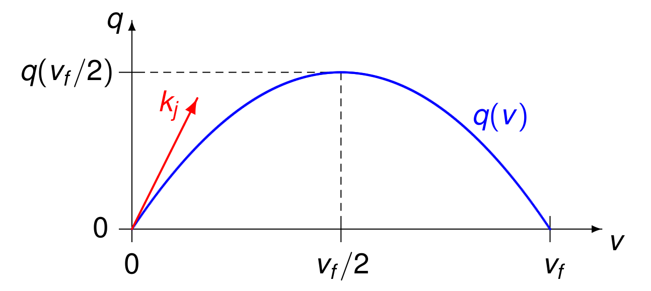
Fig. 143 Flow in function of speed.

A three dimensional model is shown in Fig. 144.

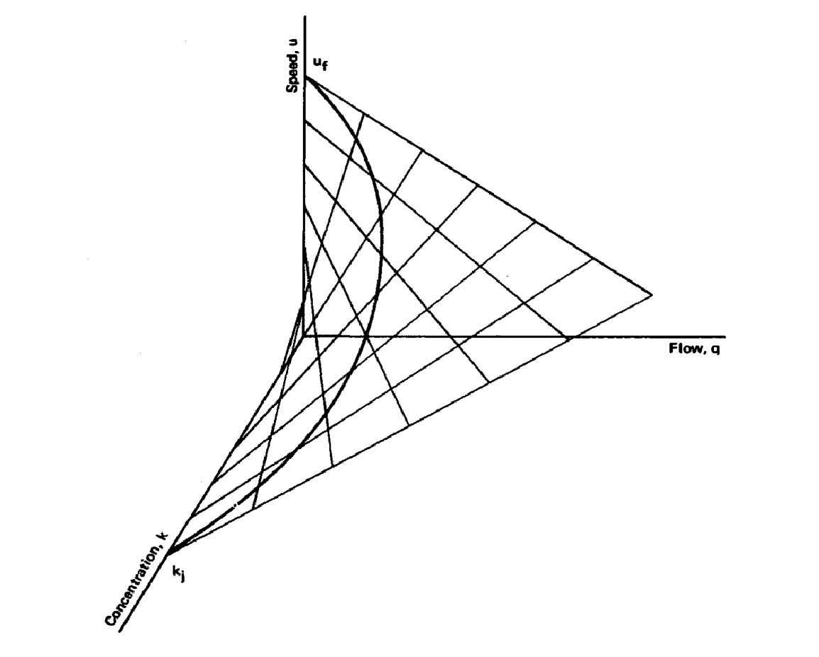
Fig. 144 Figure 4.1 in Traffic Flow Theory by D. L. Gerlough and M. J. Huber.

Accelerating Traffic Flow

The model relates speed \(v\) to flow \(q\) and concentration \(k\) as

\[v = \frac{q}{k} \quad \mbox{with units} \quad \frac{\mbox{number of cars per hour}}{\mbox{number of cars per mile}} = \frac{mile}{hour}.\]

If in the continuity equation

\[\frac{\partial q}{\partial x} + \frac{\partial k}{\partial t} = 0\]

we replace \(q\) by \(k\) times \(v\):

\[v \frac{\partial k}{\partial x} + \frac{\partial k}{\partial t} = 0,\]

then we obtain the transport equation with solution

\[k(x,t) = f(x - v t), \quad \mbox{where $f$ is the density profile at } t = 0.\]

For some constant \(C\), \(x - v t = C\) defines a characteristic curve, shown in Fig. 145

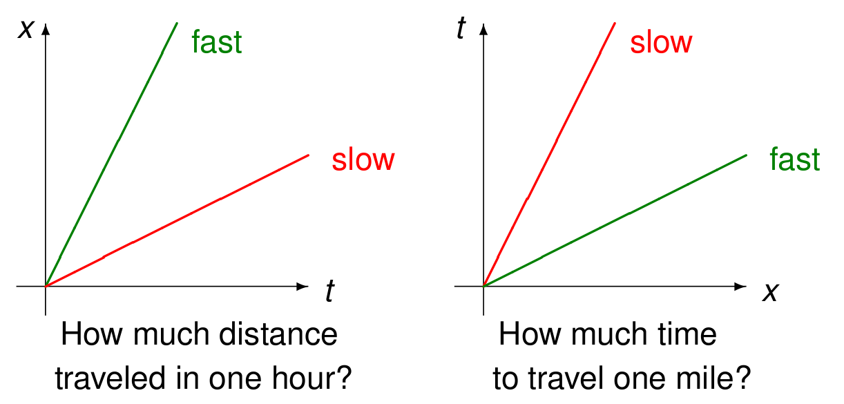
Fig. 145 Characteristic curves.

Characteristic curves can be applied to model an accelerating platoon of cars. Consider a sequence of cars.

• At \(t = t_0\), the spacing between all cars is the same.

• At \(t > t_0\), the lead car accelerates.

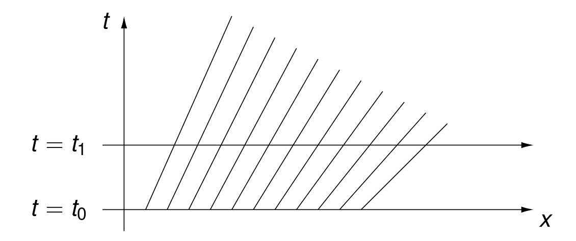
Fig. 146 Characteric curves of a platoon of cars.

In Fig. 146, at the horizontal cross sections, we see the position of each car. Observe that no two lines meet so we have no collisions.

With characteric curves, we can model what happens when a fast moving car meets a slow moving truck, as shown in Fig. 147.

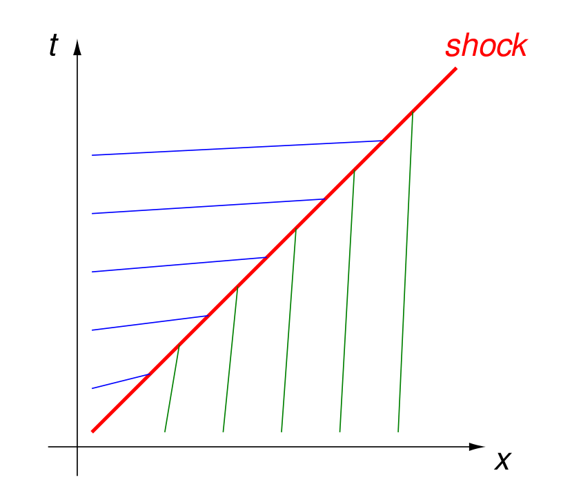
Fig. 147 A fast care meets a slow moving truck.

To model moving cars when stop light flips from red to green, we consider the transport equation with diffusion:

\[v \frac{\partial k}{\partial x} + \frac{\partial k}{\partial t} = v \alpha^2 \frac{\partial^2 k}{\partial x^2}\]

which has a traveling concentration profile as solution, shown in Fig. 148.

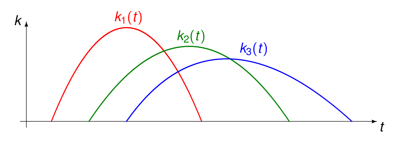
Fig. 148 Concentration profile of cars released at a traffic light.

Observe in Fig. 148:

1. \(k_1(t)\) is the concentration at the red light,

2. \(k_2(t)\) is the concentration at the green light,

3. \(k_3(t)\) is the concentration after the green light.

Proposal for a Topic of a Project

The models are experimentally verified via least squares. Apply least squares fitting on observed traffic data. Do the following:

• Collect data from an real highway.

• Fit the data for \(k(v)\) and \(q(v)\).

• Examine how realistic the models are.

In particular, can your model

• constructed with the data from one day,

• predict the traffic of the next day?

Exercises

1. Let \(\Delta x\) be one mile and \(\Delta t\) be one hour. Consider the equation

   \[\frac{\Delta q}{\Delta x} + \frac{\Delta k}{\Delta t} = 0.\]

   Verify that both terms in the equation have the same units, so the addition makes sense.

2. Let \(\Delta x\) be one mile and \(\Delta t\) be one hour. Consider the \(\Rightarrow\) in the equation

   \[\frac{\Delta q}{\Delta x} + \frac{\Delta k}{\Delta t} = 0 \quad \Rightarrow \quad q(k) = v_f k \left( \vphantom{\frac{1}{2}} 1 - \frac{k}{k_j} \right).\]

   Use the units to verify that the slope of the traffic flow equals indeed the free traffic speed at zero concentration.

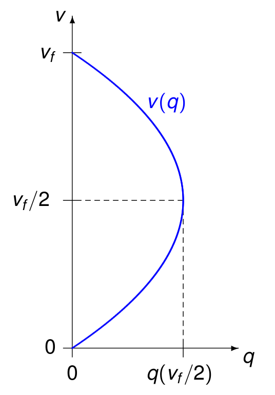
Fig. 149 Speed in function of flow.

3. Consider Fig. 149.

   1. Compute the formula for \(v(q)\).

   2. Write a paragraph to explain the picture.

4. Write one paragraph to interpret the picture in Fig. 147.

Bibliography

1. Daniel L. Gerlough and Matthew J. Huber: Traffic Flow Theory. A Monograph. Transportation Research Board Special Report 165, 1975.

2. Richard Haberman, chapter 12 on characteristic curves of Applied Partial Differential Equations with Fourier Series and Boundary Value Problems. Pearson, 2013.

3. Charles R. MacCluer, section 11.6 of Industrial Mathematics. Modeling in Industry, Science, and Government, Prentice Hall, 2000.