Modeling Vibrations by Bessel Functions

The wave equation models vibrations.

Vibrations

To model vibrations, use the wave equation \(\displaystyle \frac{\partial^2 u}{\partial t^2} = \nabla^2 u\). For example, to model a vibrating string, use:

\[\displaystyle \frac{\partial^2 u}{\partial t^2} = \frac{\partial^2 u}{\partial x^2}, \quad \mbox{for} \quad x \in [0,1], \quad t \geq 0,\]

subject to the initial conditions:

1. \(u(x, 0) = f(x)\), profile of a string,

2. \(u_t(x, 0) = 0\), no velocity,

and boundary conditions:

3. \(u(0, t) = 0\), string is fixed at the left end,

4. \(u(1, t) = 0\), string is fixed at the right end.

The method of separation of variables provides only a weak solution.

The Wave Equation

We apply the wave equation to the following situation. Strike a drum at its center and the vibrations are radially symmetric. Assuming the drum has radius one, in polar coordinates,

\[\quad u(r, t)\]

gives deviation from the equilibrium state zero, at distance \(r\) from the center of the drum, at time \(t\), starting at the strike of the drum.

As the vibrations are radially symmetric, we have a one dimensional spatial problem.

We solve the wave equation in polar coordinates

\[\frac{\partial^2 u}{\partial t^2} = \nabla^2 u % = \frac{\partial^2 u}{\partial r^2}, this is wrong! \quad 0 \leq r < 1, \quad t \geq 0,\]

with initial conditions

1. \(u(r, 0) = f(r)\), the profile of the drum at \(t = 0\), \(r < 1\),

2. \(u_t(r, 0) = 0\), we strike once, at \(t = 0\),

and boundary condition

3. \(u(1, t) = 0\), for \(t \geq 0\), the drum is fixed at end, at \(r = 1\).

In the method of the separation of variables, we propose \(U(r, t)\) as the form of the solution

\[U(r, t) = R(r) T(t),\]

where

• \(R\) is a function depending only on \(r\), and

• \(T\) is a function depending only on \(t\).

Subjecting \(U\) to the conditions of the wave equation \(\displaystyle \frac{\partial^2 u}{\partial t^2} = \nabla^2 u\) we compute

\[\frac{\partial^2 U}{\partial t^2} = R(r) \frac{\partial^2 T}{\partial t^2} \quad \mbox{and} \quad \frac{\partial^2 U}{\partial r^2} = \nabla^2 R \cdot T(t).\]

Then, seperating to the left and the right:

\[R(r) \frac{\partial^2 T}{\partial t^2} = \nabla^2 R \cdot T(t) \quad \mbox{or equivalently} \quad \frac{1}{T(t)} \frac{\partial^2 T}{\partial t^2} = \frac{1}{R(r)} \nabla^2 R.\]

The assumption of \(U(r, t) = R(r) T(t)\) for solution implies the existence of a separation constant \(\lambda\), wedged in between the equation:

\[\frac{1}{T(t)} \frac{\partial^2 T}{\partial t^2} = \lambda = \frac{1}{R(r)} \nabla^2 R.\]

We obtain two decoupled ordinary differential equations

\[\frac{\partial^2 T}{\partial t^2} = \lambda T(t),\]

and

\[\nabla^2 R = \lambda R(r).\]

What is :math:`nabla^2 R`?

For \(u = u(x,y)\), the Laplacian \(\displaystyle \nabla^2 u (x,y) = \frac{\partial^2 u}{\partial x^2} + \frac{\partial^2 u}{\partial x^2}\) in polar coordinates, for \(u = u(x = r\cos(\theta), y = r \sin(\theta))\), is

\[\nabla^2 u (r, \theta) = \frac{\partial^2 u}{\partial r^2} + \frac{1}{r} \frac{\partial u}{\partial r} + \frac{1}{r^2} \frac{\partial r^2}{\partial \theta^2}.\]

Recall exercise 3 of L-36.

For \(u = R(r)\), we then have \(\displaystyle \nabla^2 R (r) = \frac{\partial^2 R}{\partial r^2} + \frac{1}{r} \frac{\partial R}{\partial r}\) and we can write

\[\nabla^2 R = \lambda R(r) \quad \mbox{as} \quad \frac{\partial^2 R}{\partial r^2} + \frac{1}{r} \frac{\partial R}{\partial r} = \lambda R(r).\]

As a solution to

\[\frac{\partial^2 T}{\partial t^2} = - \alpha^2 T(t),\]

consider a linear combination of a cosine and a sine function:

\[\begin{split}\begin{array}{rcl} T(t) & = & a \cos(\alpha t) + b \sin(\alpha t) \\ T'(t) & = & -a~\!\alpha \sin(\alpha t) + b~\!\alpha \cos(\alpha t) \\ T''(t) & = & -a~\!\alpha^2 \cos(\alpha t) - b~\!\alpha^2 \sin(\alpha t) \\ & = & -\alpha^2 T(t). \end{array}\end{split}\]

Therefore, for some constants \(a\) and \(b\),

\[T(t) = a \cos(\alpha t) + b \sin(\alpha t)\]

is a solution to the second order differential equation.

Applying the second initial condition, subject \(T(t)\) to the second initial condition:

2. \(u_t(r, 0) = 0\), we strike once, at \(t = 0\),

which gives

\[T'(t) = - a \sin(\alpha t) + b \cos(\alpha t),\]

evaluate at \(t = 0\): \(T'(0) = b\), thus \(b = 0\), and

\[T(t) = a \cos(\alpha t).\]

Bessel Functions

The application of separation of variables in polar coordinates to the wave equation is

\[\frac{\partial^2 R}{\partial r^2} + \frac{1}{r} \frac{\partial R}{\partial r} = -\alpha^2 R,\]

or equivalently, after multiplication with \(r^2\):

\[r^2 \frac{\partial^2 R}{\partial r^2} + r \frac{\partial R}{\partial r} + r^2 \alpha^2 R = 0.\]

We eliminate \(\alpha\) by the substitution \(r = z/\alpha\):

\[\left(\frac{z^2}{\alpha^2} \right) \alpha^2 \frac{\partial^2 R}{\partial z^2} + \left( \frac{z}{\alpha} \right) \alpha \frac{\partial R}{\partial z} + \left( \frac{z^2}{\alpha^2} \right) \alpha^2 R = z^2 \frac{\partial^2 R}{\partial z^2} + z \frac{\partial R}{\partial z} + z^2 R = 0.\]

The Bessel equation

\[z^2 \frac{\partial^2 R}{\partial z^2} + z \frac{\partial R}{\partial z} + z^2 R = 0\]

has two independent solutions:

1. \(J_0\) is the Bessel function of the first kind,

2. \(Y_0\) is the Bessel function of the second kind.

We can verify this using sympy. Bessel functions in Julia are provided by the package SpecialFunctions.

Starting with the Bessel functions of the first kind:

julia> using SymPy
julia> z = Sym("z")
julia> J0 = sympy.besselj(0, z)
julia> d1J0 = J0.diff(z)
julia> d2J0 = d1J0.diff(z)

julia> odeJ0 = z^2*d2J0 + z*d1J0 + z^2*J0

julia> sympy.simplify(odeJ0)
0

This verifies symbolically that the Bessel functions of the first kind satisfy the ordinary differential equation

\[z^2 \frac{\partial^2 R}{\partial z^2} + z \frac{\partial R}{\partial z} + z^2 R = 0.\]

We contine the Julia session exploring the Bessel functions of the second kind:

julia> Y0 = sympy.bessely(0, z)
julia> d1Y0 = Y0.diff(z)
julia> d2Y0 = d1Y0.diff(z)

julia> odeY0 = z^2*d2Y0 + z*d1Y0 + z^2*Y0

julia> sympy.simplify(odeY0)
0

This verifies symbolically that the Bessel functions of the second kind satisfy the ordinary differential equation

\[z^2 \frac{\partial^2 R}{\partial z^2} + z \frac{\partial R}{\partial z} + z^2 R = 0.\]

The Bessel function of the first kind is shown in Fig. 157. We can think of \(J_0\) as a damped version of a cosine.

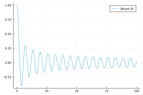
Fig. 157 The Bessel function of the first kind.

In Fig. 158, we see the Bessel function of the second kind. Observe that \(Y_0\) is no longer bounded near zero.

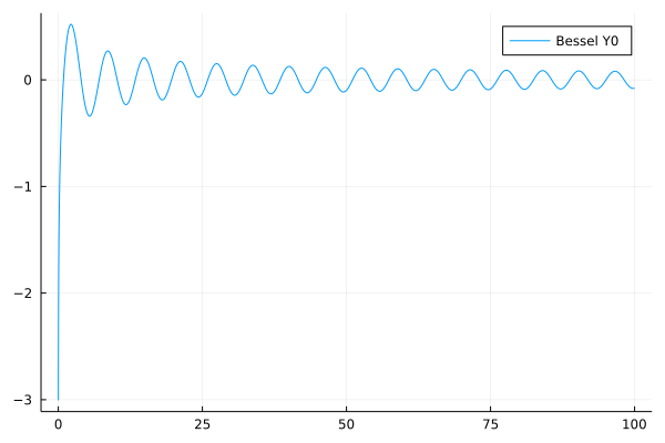
Fig. 158 The Bessel function of the second kind.

Consider the first initial condition:

1. \(u(r, 0) = f(r)\), the profile of the drum at \(t = 0\), \(r < 1\),

The solution must be bounded, so we use only \(J_0\), not \(Y_0\).

Consider the boundary condition:

2. \(u(1, t) = 0\), for \(t \geq 0\), the drum is fixed at end, at \(r = 1\).

The shape of the solution is \(U(r, t) = T(t) R(r)\), with

• \(T(t) = a \cos(\alpha t)\),

• \(R(r) = J_0(z = \alpha r)\),

thus:

\[U(r, t) = a \cos(\alpha t) J_0(\alpha r).\]

The condition \(u(1, t) = 0\) gives, setting \(r = 1\):

\[\underbrace{a \cos(\alpha t)}_{\not= 0} J_0(\alpha) = 0 \quad \Rightarrow \quad J_0(\alpha) = 0.\]

The first ten roots are computed as follows.

julia> using FastGaussQuadrature

julia> roots = approx_besselroots(0.0, 10)
10-element Vector{Float64}:
 2.404825557695773
 5.520078110286311
 8.653727912911013
11.791534439014281
14.930917708487785
18.071063967910924
21.21163662987926
24.352471530749302
27.493479132040253
30.634606468431976

julia>

Now we derive the general solution. For every root \(\alpha_n$ of $J_0\), we have a solution of the form

\[U_n(r, t) = a_n \cos(\alpha_n t) J_0(\alpha_n r).\]

Viewing \(U_n\) as a basis of functions, we have the general solution

\[U(r, t) = \sum_{n=1}^\infty a_n \cos(\alpha_n t) J_0(\alpha_n r).\]

To determine the coefficients \(a_n\), use the condition

1. \(u(r, 0) = f(r)\), the profile of the drum at \(t = 0\), \(r < 1\).

As before, we are using an orthogonal basis.

Applying \(u(r, 0) = f(r)\) to \(\displaystyle U(r, t) = \sum_{n=1}^\infty a_n \cos(\alpha_n t) J_0(\alpha_n r)\) yields

\[U(r, 0) = \sum_{n=1}^\infty a_n J_0(\alpha_n r) = f(r).\]

With the inner product

\[\big\langle f(r), g(r) \big\rangle = \int_0^1 f(r)~\!g(r)~\!r~\!dr.\]

we have

\[\big\langle J_0(\alpha_n r), J_0(\alpha_m r) \big\rangle = 0, \quad \mbox{for } n \not= m.\]

By \(\displaystyle \big\langle J_0(\alpha_n r), J_0(\alpha_m r) \big\rangle = 0\), for \(n \not= m\),

\[\begin{split}\begin{array}{rcl} {\displaystyle \big\langle f(r), J_0(\alpha_m r) \big\rangle} & = & {\displaystyle \big\langle \sum_{n=1}^\infty a_n J_0(\alpha_n r) , J_0(\alpha_m r) \big\rangle} \\ & = & {\displaystyle a_m ~ \big\langle J_0(\alpha_m r) , J_0(\alpha_m r) \big\rangle}. \end{array}\end{split}\]

The coefficients \(a_m\) are computed as

\[a_m = \frac{\big\langle f(r), J_0(\alpha_m r) \big\rangle} {\big\langle J_0(\alpha_m r) , J_0(\alpha_m r) \big\rangle}.\]

Proposal for a Topic of a Project

Can you hear the shape of a drum? is the title of the paper by Mark Kac, published in April 1966 by The American Mathematical Monthly, pages 1-23.

This problem is still open, according to the paper Can’t One Really Hear the Shape of a Drum? by S. Zuluaga and F. Fonseca, in Acoustical Physics, Vol. 57, No. 4, pages 465–472, 2011.

• Study the papers and illustrate the importance of this problem for industrial applications.

• Summarize the findings of the two papers.

Exercises

1. Use the method of characteristic lines to show that

   \[u(x, t) = f(x - c t) + g(x + c t)\]

   satisfies the one dimensional wave equation

   \[\displaystyle \frac{\partial^2 u}{\partial t^2} = c^2 \frac{\partial^2 u}{\partial x^2}, \quad \mbox{for} \quad x \in [0,1], \quad t \geq 0,\]

   where \(c\) is the wave speed. The functions \(f\) and \(g\) are determined within constants that sum to zero.

2. Consider the Bessel functions \(J_n\), for \(n=0,1,2,3,4\).

   Make a plot of \(J_n(z)\), for \(z \in [0,1]\), and for \(n=0,1,2,3,4\).

   What do you observe about the roots of those five functions?

3. Verify the orthogonality numerically for \(J_0(\alpha_n r)\) for \(n = 1, 2, 3, 4, 5\).

4. For a square drum, for \(x \in [0,1]\) and \(y \in [0,1]\), use the proposed solution

   \[u(x, y, t) = \sum_{m=1}^\infty \sum_{n=1}^\infty c_{m,n} \cos\left(\pi t \sqrt{m^2 + n^2}\right) \sin(m \pi x) \sin(n \pi y).\]

   1. Define the partial differential equation, with all initial and boundary conditions for the square drum.

   2. Interpret the solution and argue why this proposal makes sense.

   3. How are the coefficients \(c_{m,n}\) computed?

Bibliography

1. Charles R. MacCluer, problem 5 of chapter 11 of Industrial Mathematics. Modeling in Industry, Science, and Government, Prentice Hall, 2000.