Evaluating Parallel Performance

When evaluating the performance of parallel programs, we start by measuring time. We distinguish between times directly from time measurements and those that are derived, e.g.: flops. When the number of processors grows, the size of the problem has to grow as well to achieve the same performance, which then leads to the notion of isoefficiency. For task based parallel programs the length of a critical path in a task graph provides an upper bound on the speedup. With the roofline model, we can distinguish between computations that are compute bound or memory bound.

Metrics

The goal is to characterize parallel performance. Metrics are determined from performance measures. Time metrics are obtained from time measurements.

Time measurements are

1. execution time which includes

   • CPU time and system time

   • I/O time

2. overhead time is caused by

   • communication

   • synchronization

The wall clock time measures execution time plus overhead time.

Time metrics come directly from time measurements. Derived metrics are results of arithmetical metric expressions.

Definition of flops

flops are the number of floating-point operations per second:

\[\frac{\mbox{number of floating-point operations done}} {\mbox{execution time}}.\]

Definition of communication-to-computation ratio:

The communication-to-computation ratio is

\[\frac{\mbox{communication time}}{\mbox{execution time}}.\]

Definition of memory access-to-computation ratio:

The memory access-to-computation ratio is

\[\frac{\mbox{time spent on memory operations}}{\mbox{execution time}}.\]

Speedup and efficiency depend on the number of processors and are called parallelism metrics. Metrics used in performance evaluation are

• Peak speed is the maximum flops a computer can attain. Fast Graphics Processing Units achieve teraflop performance.

• Benchmark metrics use representative applications. The LINPACK benchmark ranks the Top 500 supercomputers.

• Tuning metrics include bottleneck analysis. For task-based parallel programs, the application of critical path analysis techniques finds the longest path in the execution of a parallel program.

Isoefficiency

The notion of isoefficiency complements the scalabiliy treatments introduced by the laws of Ahmdahl and Gustafson. The law of Ahmdahl keeps the dimension of the problem fixed and increases the number of processors. In applying the law of Gustafson we do the opposite: we fix the number of processors and increase the dimension of the problem. In practice, to examine the scalability of a parallel program, we have to treat both the dimension and the number of processors as variables.

Before we examine how relates to scalability, recall some definitions. For p processors:

\[{\rm Speedup} = \frac{\rm serial~time}{\rm parallel~time} = S(p) \rightarrow p.\]

As we desire the speedup to reach p, the efficiency goes to 1:

\[{\rm Efficiency} = \frac{\rm Speedup}{p} = \frac{S(p)}{p} = E(p) \rightarrow 1.\]

Let \(T_s\) denote the serial time, \(T_p\) the parallel time, and \(T_0\) the overhead, then: \(p T_p = T_s + T_0\).

\[E(p) = \frac{T_s}{p T_p} = \frac{T_s}{T_s + T_0} = \frac{1}{1 + T_0/T_s}\]

The scalability analysis of a parallel algorithm measures its capacity to effectively utilize an increasing number of processors.

Let \(W\) be the problem size, for FFT: \(W = n \log(n)\). Let us then relate \(E\) to \(W\) and \(T_0\). The overhead \(T_0\) depends on \(W\) and \(p\): \(T_0 = T_0(W,p)\). The parallel time equals

\[T_p = \frac{W + T_0(W,p)}{p}, \quad \mbox{ Speedup } S(p) = \frac{W}{T_p} = \frac{W p}{W + T_0(W,p)}.\]

The efficiency is

\[E(p) = \frac{S(p)}{p} = \frac{W}{W + T_0(W,p)} = \frac{1}{1 + T_0(W,p)/W}.\]

The goal is for \(E(p) \rightarrow 1$ as $p \rightarrow \infty\). The algorithm scales badly if W must grow exponentially to keep efficiency from dropping. If W needs to grow only moderately to keep the overhead in check, then the algorithm scales well.

Isoefficiency relates work to overhead:

\[\begin{split}\begin{array}{rcl} {\displaystyle E = \frac{1}{1 + T_0(W,p)/W}} & \Rightarrow & {\displaystyle \frac{1}{E} = \frac{1 + T_0(W,p)/W}{1}} \\ & \Rightarrow & {\displaystyle \frac{1}{E} - 1 = \frac{T_0(W,p)}{W}} \\ & \Rightarrow & {\displaystyle \frac{1-E}{E} = \frac{T_0(W,p)}{W}}. \end{array}\end{split}\]

The isoefficiency function is

\[W = \left( \frac{E}{1-E} \right) T_0(W,p) \quad {\rm or} \quad W = K ~\! T_0(W,p).\]

Keeping K constant, isoefficiency relates W to \(T_0\). We can relate isoefficiency to the laws we encountered earlier:

• Amdahl’s Law: keep W fixed and let p grow.

• Gustafson’s Law: keep p fixed and let W grow.

Let us apply the isoefficiency to the parallel FFT. The isoefficiency function: \(W = K~\! T_0(W,p)\). For FFT: \(T_s = n \log(n) t_c\), where \(t_c\) is the time for complex multiplication and adding a pair. Let \(t_s\) denote the startup cost and \(t_w\) denote the time to transfer a word. The time for a parallel FFT:

\[T_p = \underbrace{t_c \left( \frac{n}{p} \right) \log(n)}_{\mbox{computation time}} + \underbrace{t_s \log(p)}_{\mbox{start up time}} + \underbrace{t_w \left( \frac{n}{p} \right) \log(p)}_{\mbox{transfer time}}.\]

Comparing start up cost to computation cost, using the expression for \(T_p\) in the efficiency \(E(p)\):

\[\begin{split}\begin{array}{rcl} {\displaystyle E(p) = \frac{T_s}{p T_p}} & = & {\displaystyle \frac{n \log(n) t_c}{n \log(n) t_c + p \log(p) t_s + n \log(p) t_w}} \\ & = & {\displaystyle \frac{W t_c}{W t_c + p \log(p) t_s + n \log(p) t_w}, ~~ W = n \log(n)}. \end{array}\end{split}\]

Assume \(t_w = 0\) (shared memory):

\[E(p) = \frac{W t_c}{W t_c + p \log(p) t_s}.\]

We want to express \(\displaystyle K = \frac{E}{1-E}\), using \(\displaystyle \frac{1}{K} = \frac{1-E}{E} = \frac{1}{E} - 1\):

\[\frac{1}{K} = \frac{W t_c + p \log(p) t_s}{W t_c} - \frac{W t_c}{W t_c} \quad \Rightarrow \quad W = K \left( \frac{t_s}{t_c} \right) p \log(p).\]

The plot in Fig. 38 shows by how much the work load must increase to keep the same efficiency for an increasing number of processors.

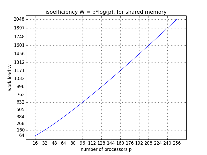
Fig. 38 Isoefficiency for a shared memory application.

Comparing transfer cost to the computation cost, taking another look at the efficiency \(E(p)\):

\[E(p) = \frac{W t_c}{W t_c + p \log(p) t_s + n \log(p) t_w}, \quad W = n \log(n).\]

Assuming \(t_s = 0\) (no start up):

\[E(p) = \frac{W t_c}{W t_c + n \log(p) t_w}.\]

We want to express \(\displaystyle K = \frac{E}{1-E}\), using \(\displaystyle \frac{1}{K} = \frac{1-E}{E} = \frac{1}{E} - 1\):

\[\frac{1}{K} = \frac{W t_c + n \log(p) t_w}{W t_c} - \frac{W t_c}{W t_c} \quad \Rightarrow \quad W = K \left( \frac{t_w}{t_c} \right) n \log(p).\]

In Fig. 39 the efficiency function is displayed for an increasing number of processors and various values of the dimension.

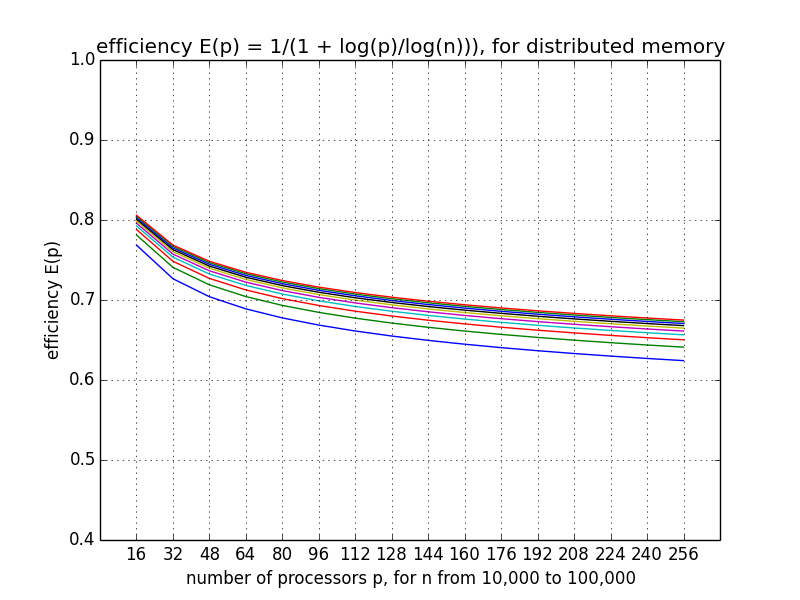
Fig. 39 Scalability analysis with a plot of the efficiency function.

Task Graph Scheduling

A task graph is a Directed Acyclic Graph (DAG):

• nodes are tasks, and

• edges are precedence constraints between tasks.

Task graph scheduling or DAG scheduling maps the task graph onto a target platform.

The scheduler

1. takes a task graph as input,

2. decides which processor will execute what task,

3. with the objective to minimize the total execution time.

Let us consider the task graph of forward substitution.

Consider \(L {\bf x} = {\bf b}\), an \(n\)-by-\(n\) lower triangular linear system, where \(L = [\ell_{i,j}] \in {\mathbb R}^{n \times n}\), \(\ell_{i,i} \not= 0\), \(\ell_{i,j} = 0\), for \(j > i\).

For \(n = 3\), we compute:

\[\begin{split}\begin{array}{lclcl} \ell_{1,1} x_1 & \!=\! & b_1 & \Rightarrow & x_1 := b_1/\ell_{1,1} \\ \ell_{2,1} x_1 + \ell_{2,2} x_2 & \!=\! & b_2 & \Rightarrow & x_2 := (b_2 - \ell_{2,1} x_1)/\ell_{2,2} \\ \ell_{3,1} x_1 + \ell_{3,2} x_2 + \ell_{3,3} x_3 & \!=\! & b_3 & \Rightarrow & x_3 := (b_3 - \ell_{3,1} x_1 - \ell_{3,2} x_2)/\ell_{3,3} \end{array}\end{split}\]

The formulas translate into pseudo code, with tasks labeled for each instruction:

\[\begin{split}\begin{array}{l} \mbox{\em task } T_{1,1}: x_1 := b_1/\ell_{1,1} \\ \mbox{for } i \mbox{ from } 2 \mbox{ to } n \mbox{ do} \\ \quad \mbox{for } j \mbox{ from } 1 \mbox{ to } i-1 \mbox{ do} \\ \qquad \mbox{\em task } T_{i,j}: b_i := b_i - \ell_{i,j} x_j \\ \quad \mbox{\em task } T_{i,i}: x_i := b_i/\ell_{i,i} \end{array}\end{split}\]

To decide which tasks depend on which other tasks, we apply Bernstein’s conditions.

Each task \(T\) has an input set \(\mbox{\rm in}(T)\), and an output set \(\mbox{\rm out}(T)\).

Tasks \(T_1\) and \(T_2\) are independent if

\[\begin{split}\begin{array}{rcl} \mbox{\rm in}(T_1) ~\cap~ \mbox{\rm out}(T_2) & = & \emptyset, \mbox{ and} \\ \mbox{\rm out}(T_1) ~\cap~ \mbox{\rm in}(T_2) & = & \emptyset, \mbox{ and} \\ \mbox{\rm out}(T_1) ~\cap~ \mbox{\rm out}(T_2) & = & \emptyset. \end{array}\end{split}\]

Applied to forward substitution:

\[\begin{split}\begin{array}{lcl} \mbox{\em task } T_{1,1}: x_1 := b_1/\ell_{1,1} & & \mbox{\rm in}(T_{1,1}) = \{ b_1, \ell_{1,1} \}, \mbox{\rm out}(T_{1,1}) = \{ x_1 \} \\ \mbox{for } i \mbox{ from } 2 \mbox{ to } n \mbox{ do} & & \\ \quad \mbox{for } j \mbox{ from } 1 \mbox{ to } i-1 \mbox{ do} & & \\ \qquad \mbox{\em task } T_{i,j}: b_i := b_i - \ell_{i,j} x_j & & \mbox{\rm in}(T_{i,j}) = \{ x_j, b_i, \ell_{i,j} \}, \mbox{\rm out}(T_{i,j}) = \{ b_i \} \\ \quad \mbox{\em task } T_{i,i}: x_i := b_i/\ell_{i,i} & & \mbox{\rm in}(T_{i,i}) = \{ b_i, \ell_{i,i} \}, \mbox{\rm out}(T_{i,i}) = \{ x_i \} \end{array}\end{split}\]

The task graph for a four dimensional linear system is shown in Fig. 40.

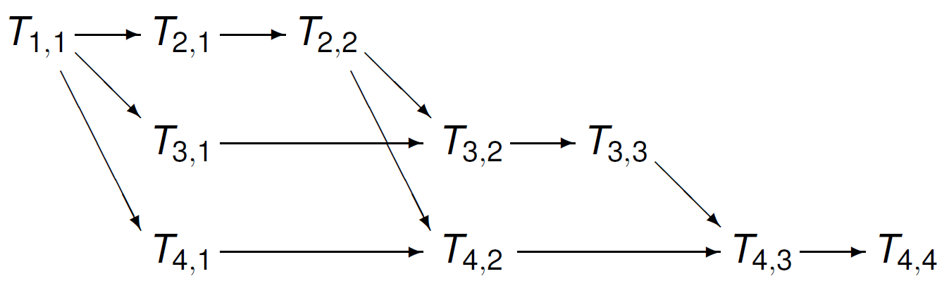
Fig. 40 Task graph for forward substition to solve a four dimensional lower triangular linear system.

In the task graph of Fig. 40, a critical path is colored in red in Fig. 41.

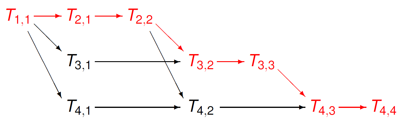
Fig. 41 A critical path is shown in red in the task graph for forward substition to solve a four dimensional lower triangular linear system.

Recall that \(T_{i,i}\) computes \(x_i\). The length of a critical path limits the speedup. For the above example, a sequential execution

\[T_{1,1}, T_{2,1}, T_{3,1}, T_{4,1}, T_{2,2}, T_{3,2}, T_{4,2}, T_{3,3}, T_{4,3}, T_{4,4}\]

takes 10 steps. The length of a critical path is 7. At most three threads can compute simultaneously. For \(n=4\), we found 7. For \(n=5\), the length of the critical path is 9, as can be seen from Fig. 42.

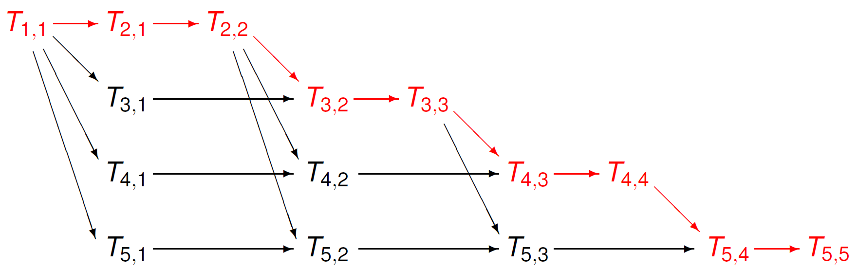
Fig. 42 A critical path is shown in red in the task graph for forward substition to solve a five dimensional lower triangular linear system.

For any dimension \(n\), the length of the critical path is \(2n-1\). At most \(n-1\) threads can compute simultaneously.

The Roofline Model

Performance is typically measured in flops: the number of floating-point operations per second.

Definition of arithmetic intensity

The arithmetic intensity of a computation is the number of floating-point operations per byte.

For example, consider \(z := x + y\), assign \(x+y\) to \(z\). One floating point operation involving 64-bit doubles, and each double occupies 8 bytes, so the arithmetic intensity is \(1/24\).

Do you want faster memory or faster processors? To answer this question, we must decide if the computation if memory bound or compute bound.

Definition of memory bound

A computation is memory bound if the peak memory bandwidth determines the performance.

Memory bandwidth is the number of bytes per second that can be read or stored in memory.

Definition of compute bound

A computation is compute bound if the peak floating-point performance determines the performance.

A high arithmetic intensity is needed for a compute bound computation.

As an introduction to the roofline model, consider Fig. 43. The formula for attainable performance is

\[\begin{split}\begin{array}{c} \mbox{attainable} \\ \mbox{GFlops/sec} \end{array} = \min \left\{ \begin{array}{c} \mbox{peak floating point performance} \\ \\ \mbox{peak memory bandwidth} \times \mbox{operational intensity} \end{array} \right.\end{split}\]

Observe the difference between arithmetic and operational intensity:

• arithmetic intensity measures the number of floating point operations per byte,

• operational intensity measures the number of operations per byte.

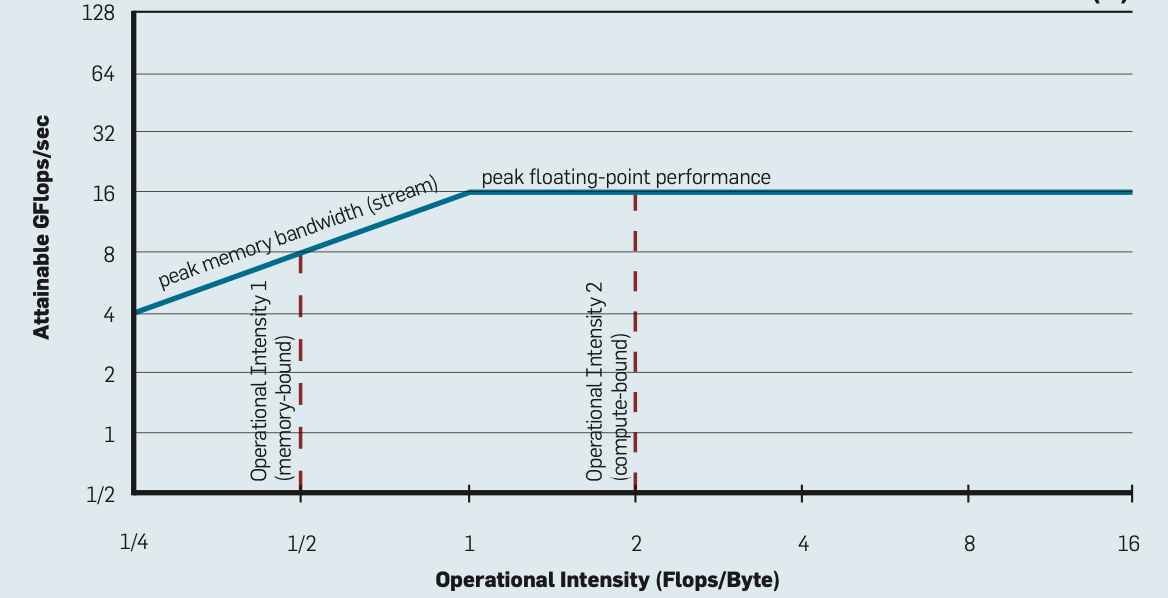
Fig. 43 The roofline model. Image copied from the paper by S. Williams, A. Waterman, and D. Patterson, 2009.

In applying the roofline model, in Fig. 43,

1. The horizontal line is the theoretical peak performance, expressed in gigaflops per second, the units of the vertical axis.

2. The units of the horizontal coordinate axis are flops per byte.

   The ridge point is the ratio of the theoretical peak performance and the memory bandwidth.

3. For any particular computation, record the pair \((x, y)\)

   1. \(x\) is the arithmetic intensity, number of flops per byte,

   2. \(y\) is the performance defined by the number of flops per second.

If \((x,y)\) lies under the horizontal part of the roof, then the computation is compute bound, otherwise, the computation is memory bound.

To summarize, to decide if a computation is memory bound or compute bound, consider Fig. 44.

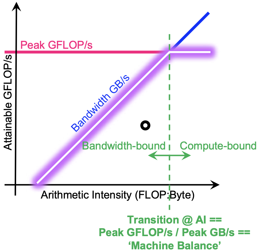
Fig. 44 Memory bound or compute bound? Image copied from the tutorial slides by Charlene Yang, LBNL, 16 June 2019.

Bibliography

1. Thomas Decker and Werner Krandick: On the Isoefficiency of the Parallel Descartes Method. In Symbolic Algebraic Methods and Verification Methods, pages 55–67, Springer 2001. Edited by G. Alefeld, J. Rohn, S. Rump, and T. Yamamoto.

2. Ananth Grama, Anshul Gupta, George Karypis, Vipin Kumar: Introduction to Parallel Computing. 2nd edition, Pearson 2003.

3. Vipin Kumar and Anshul Gupta: Analyzing Scalability of Parallel Algorithms and Architectures. Journal of Parallel and Distributed Computing 22: 379–391, 1994.

4. Alan D. Malony: Metrics. In Encycopedia of Parallel Computing, edited by David Padua, pages 1124–1130, Springer 2011.

5. Yves Robert: Task Graph Scheduling. In Encycopedia of Parallel Computing, edited by David Padua, pages 2013–2024, Springer 2011.

6. S. Williams, A. Waterman, and D. Patterson: Roofline: an insightful visual performance model for multicore architectures. Communications of the ACM, 52(4):65-76, 2009.