GPU Accelerated QR
The Householder QR is rich in matrix matrix multiplication, an operation that can be accelerated very well by GPUs.
Householder Reflectors
Proof. The vector \({\bf x} - {\bf y}\) is perpendicular to \({\bf x} + {\bf y}\) if \(({\bf x} - {\bf y})^T ({\bf x} + {\bf y}) = 0\).
Q.E.D.
The Lemma is used to define a projection operator. For a nonzero vector \(\bf z\), consider \(\displaystyle P = \frac{{\bf z} {\bf z}^T}{{\bf z}^T {\bf z}}\).
Observe:
If \(\bf z\) is a n-by-1 column vector, then \({\bf z}^T\) is a 1-by-n row vector, and \({\bf z} {\bf z}^T\) is n-by-n.
\({\bf z}^T {\bf z} = \|{\bf z}\|_2^2\).
\(P\) is a projection operator, with the property \(P^2 = P\).
\(H\) is an orthogonal matrix: \(H^T H = I\).
Denote \(\displaystyle P = \frac{{\bf z} {\bf z}^T}{{\bf z}^T {\bf z}}\), then \(H = I - 2P\).
because \(P^2 = P\).
Since \(P\) is symmetric, \(H\) is symmetric too.
Now we get to the reflector property.
Given two nonzero vectors \(\bf x\) and \(\bf y\): \(\|{\bf x}\|_2 = \|{\bf y}\|_2\) and \({\bf z} = {\bf y} - {\bf x} \not= {\bf 0}\).
The Householder reflector \(\displaystyle H = I - 2 \frac{{\bf z} {\bf z}^T}{{\bf z}^T {\bf z}}\) has the property \(H {\bf x} = {\bf y}\).
A geometric interpretation is shown in Fig. 137.
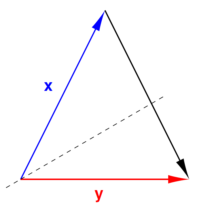
Fig. 137 Let \({\bf y} = H {\bf x} = {\bf x} - 2 P {\bf x}\), then the reflection through the bisector brings \(\bf x\) to \(\bf y\).
The Householder QR computes the QR factorization with Householder reflectors. Consider a 3-by-2 matrix \(A = [{\bf a}_1 ~ {\bf a}_2]\).
Compute \(H_1\) so that
\[\begin{split}H_1 {\bf a}_1 = \left[ \begin{array}{c} a_{1,1}/\|{\bf a}_1 \|_2 \\ 0 \\ 0 \end{array} \right].\end{split}\]Let \({\bf b}_2 = H_1 {\bf a}_2\) and select
\[\begin{split}{\bf c} = \left[ \begin{array}{c} b_{2} \\ b_{3} \end{array} \right].\end{split}\]Compute \(H_2\) so that
\[\begin{split}H_2 {\bf c} = \left[ \begin{array}{c} c_1/\|{\bf c}\|_2 \\ 0 \end{array} \right].\end{split}\]
Then \(H_2 H_1 A\) is an upper triangular matrix \(R\).
Recall that \(H\) is orthogonal and symmetric: \(H^{-1} = H^T = H\).
On a 4-by-4 matrix, the evolution of the structure of the matrix during the QR factorization is illustrated in Fig. 138.
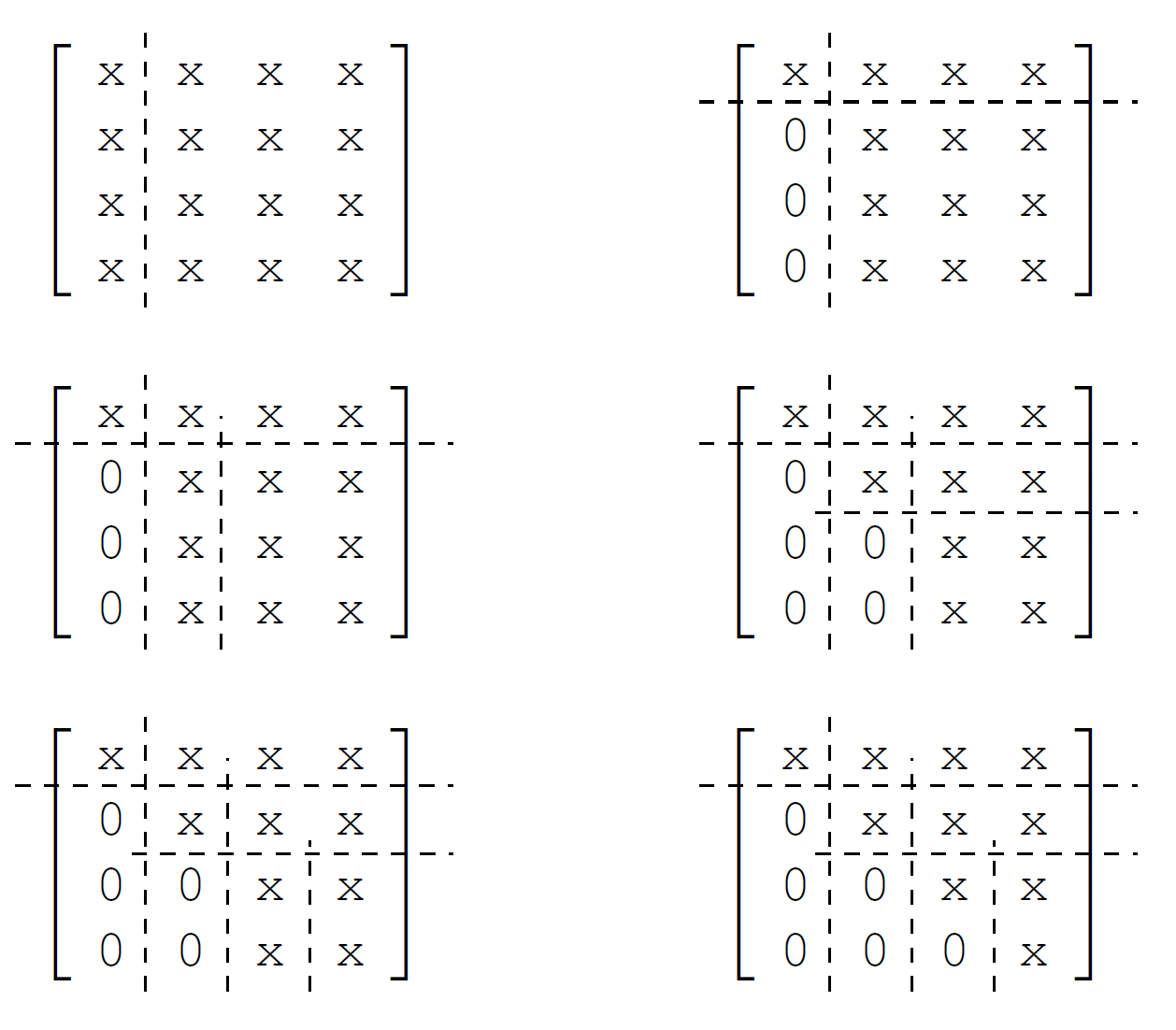
Fig. 138 Evolution of the structure a 4-by-4 matrix in the Householder QR.
Code to compute the Householder vector \({\bf v}\), \(P = I - \beta {\bf v} {\bf v}^T\) is defined in the Julia function below.
"""
    house(x::Array{Float64,1})

returns the Householder vector and the beta.
"""
function house(x::Array{Float64,1})
    n = length(x)
    y = x[2:n]
    sigma = y'*y
    v = [1; y]
    if(sigma == 0)
        beta = 0
    else
        mu = sqrt(x[1]^2 + sigma)
        if x[1] <= 0
            v[1] = x[1] - mu
        else
            v[1] = -sigma/(x[1] + mu)
        end
        beta = 2*v[1]^2/(sigma + v[1]^2)
        v = v/v[1]
    end
    return v, beta
end
Then the Householder QR is defined in the following Julia function:
"""
    houseQR(A::Array{Float64,2})

returns the Q and R of the QR.
"""
function houseQR(A::Array{Float64,2})
    m = size(A,1)
    n = size(A,2)
    R = deepcopy(A)
    Q = Matrix{Float64}(I,m,m)
    for k = 1:n
        v, b = house(R[k:m,k])
        R[k:m,k:n] = R[k:m,k:n] - b*v*v'*R[k:m,k:n]
        Q[1:m,k:m] = Q[1:m,k:m] - b*Q[1:m,k:m]*v*v'
    end
    return Q, R
end
The blocked Householder QR uses the WY representation, which will be introduced next.
Consider a \(3m\)-by-\(3n\) tiled matrix, \(m \geq n\), as in Fig. 139.
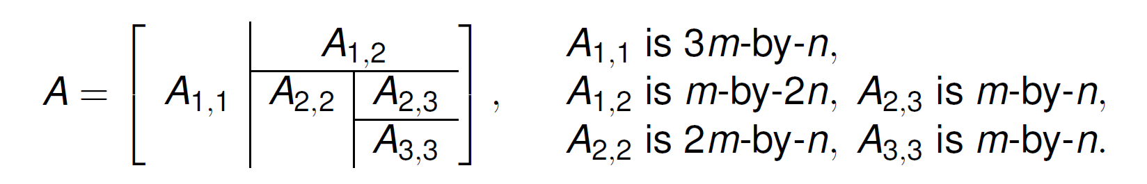
Fig. 139 A \(3m\)-by-\(3n\) tiled matrix.
The Householder transformations are accumulated in an orthogonal \(3m\)-by-\(3m\) matrix \(Q\). The upper triangular reduction \(R\) of \(A\) is written in the matrix \(A\).
Two main references:
C. Bishof and C.F. Van Loan: The WY representation for products of Householder matrices. SIAM J.Sci.Stat.Comput. 8(1):s1–s13, 1987.
Matrix Computations by G.H. Golub and C.F. Van Loan, 1996.
The evolution of \(Q\) and \(R\), where \(I\) is the identity matrix is shown in Fig. 140.
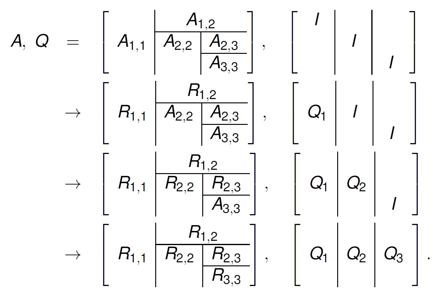
Fig. 140 Evolution of the tiled matrix during the QR factorization.
The Householder reflector \(P\) is represented by a vector \(\bf v\):
where \(\bf x\) is the current column and \({\bf e}_1 = (1,0,\ldots,0)^T\).
The Householder matrices are aggregated in an orthogonal matrix
where \(Y\) stores the Householder vectors in a trapezoidal shape; \(W\) is defined by the Householder vectors and the corresponding \(\beta\) coefficients. With this WY representation, the updates to \(Q\) and \(R\) are
which involve many matrix-matrix products.
Multiple Doubles on Graphics Processing Units
For example, the 2-norm of a vector of dimension 64 of random complex numbers on the unit circle equals 8. Observe the second double:
double double : 8.00000000000000E+00 - 6.47112461314111E-32
  quad double : 8.00000000000000E+00 + 3.20475411419393E-65
  octo double : 8.00000000000000E+00 - 9.72609915198313E-129
If the result fits a 64-bit double, then the second double represents the accuracy of the result. Multiple double arithmetic is therefore sometimes referred to as error free transformations.
Two advantages are
predictable overhead, cost of double double \(\approx\) complex double,
exploits hardware double arithmetic.
However, be aware of the disavantages:
not true multiprecision, fixed multiples of bits in fractions,
infinitesimal computations not possible because of fixed exponent.
One motivation is power series arithmetic. Consider the following expansion:
Assuming the quadratic convergence of Newton’s method, Table 34 motivates the need for multiple double precision, to accurately represent the last coefficient in the series.
\(k\) |
\(1/k!\) |
recommended precision |
|
|---|---|---|---|
7 |
|
double precision okay |
|
15 |
|
use double doubles |
|
23 |
|
use double doubles |
|
31 |
|
use quad doubles |
|
47 |
|
use octo doubles |
|
63 |
|
use octo doubles |
|
95 |
|
need hexa doubles |
|
127 |
|
need hexa doubles |
Software packages to implement multiple double precision are:
QDlib by Y. Hida, X. S. Li, and D. H. Bailey. Algorithms for quad-double precision floating point arithmetic. In the Proceedings of the 15th IEEE Symposium on Computer Arithmetic, pages 155–162, 2001.
GQD by M. Lu, B. He, and Q. Luo. Supporting extended precision on graphics processors. In the Proceedings of the Sixth International Workshop on Data Management on New Hardware (DaMoN 2010), pages 19–26, 2010.
CAMPARY by M. Joldes, J.-M. Muller, V. Popescu, and W. Tucker. CAMPARY: Cuda Multiple Precision Arithmetic Library and Applications. In Mathematical Software – ICMS 2016, the 5th International Conference on Mathematical Software, pages 232–240, Springer-Verlag, 2016.
The number of floating-point operations for multiple double arithmetic are cost overhead factors are listed in Table 35.
\(+\) |
\(\star\) |
\(/\) |
average |
|
|---|---|---|---|---|
double double |
20 |
32 |
70 |
37.7 |
quad double |
89 |
336 |
893 |
439.3 |
octo double |
269 |
1742 |
5126 |
2379.0 |
Teraflop performance compensates the overhead of quad doubles.
NVIDIA GPU |
CUDA |
#MP |
#cores/MP |
#cores |
GHz |
|---|---|---|---|---|---|
Pascal P100 |
6.0 |
56 |
64 |
3584 |
1.33 |
Volta V100 |
7.0 |
80 |
64 |
5120 |
1.91 |
GeForce RTX 2080 |
7.5 |
46 |
64 |
2944 |
1.10 |
The double precision peak performance of the P100 is 4.7 TFLOPS. At 7.9 TFLOPS, the V100 is 1.68 times faster than the P100.
The code for the arithmetical operations generated by the CAMPARY software was customized for each precision.
Instead of representing a quad double by an array of four doubles, all arithmetical operations work on four separate variables, one for each double.
By this customization an array of quad doubles is stored as four separate arrays of doubles and a matrix of quad doubles is represented by four matrices of doubles.
The
double2anddouble4types of the CUDA SDK work for double double and quad double, but not for the more general multiple double arithmetic.QDlib provides definitions for the square roots and various other useful functions for double double and quad double arithmetic.
Those definitions are extended up to octo double precision.
Consider for example the computation of the 2-norm of a vector of complex numbers, given in \(\bf z = (z_1, z_2, \ldots, z_n)\).
For small \(n\), only one block of threads is launched.
The prefix sum algorithm proceeds in \(\log_2(n)\) steps.
For large \(n\), subsums are accumulated for each block.
Specific for the accelerated multiple double implementation:
The size of shared memory needs to be set for each precision.
\(\sqrt{~}\) applies Newton’s method for staggered precisions.
The use of registers increases as the precision increases \(\ldots\)
Accelerated Blocked Householder QR
Early GPU implementations were reported in
Baboulin, Dongarra, and Tomov, TR UT-CS-08-200, 2008
Kerr, Campbell, and Richards, GPGPU’09 conference
Volkov and Demmel, Conference on Supercomputing, 2008
The algorithm operates in four stages and is implemented by several kernels. Its specification is listed in Table 37.
I/O |
parameter description |
|---|---|
Input |
\(N\) is the number of tiles |
\(n\) is the size of each tile |
|
\(M\) is the number of rows, \(M \geq N n\) |
|
\(A\) is an \(M\)-by-\(Nn\) matrix |
|
Output |
\(Q\) is an orthogonal \(M\)-by-\(M\) matrix |
\(R\) is an \(M\)-by-\(Nn\) matrix \(A = Q R\) |
The algorithm then runs as follows:
For k from 1 to \(N\) do
Compute Householder vectors for one tile, reduce \(R_{k,k}\).
Define \(Y\), compute \(W\) and \(Y \star W^T\).
Add \(Q \star YW^T\) to update \(Q\).
If \(k < N\), add \(YW^T\star C\) to update \(R\).
The code is written for multiple double precision. At <github.com/janverschelde/PHCpack>, GPL-3.0 License.
Thanks to the high Compute to Global Memory Access ratios of multiple double precision, entries of a matrix can be loaded directly into the registers of a kernel (bypassing shared memory).
The computation cost is proportional to \(M^3\), for \(M = Nn\). The hope is to reduce the cost by a factor of \(M\).
Concerning the data staging, a matrix \(A\) of multiple doubles is stored as \([A_1, A_2, \ldots, A_m]\),
\(A_1\) holds the most significant doubles of \(A\),
\(A_m\) holds the least significant doubles of \(A\).
Similarly, \(\bf b\) is an array of \(m\) arrays \([{\bf b}_1, {\bf b}_2, \ldots, {\bf b}_m]\), sorted in the order of significance.
In complex data, real and imaginary parts are stored separately.
The main advantages of this representation are twofold:
facilitates staggered application of multiple double arithmetic,
benefits efficient memory coalescing, as adjacent threads in one block of threads read/write adjacent data in memory, avoiding bank conflicts.
About the input matrices:
Random numbers are generated for the input matrices.
Condition numbers of random triangular matrices almost surely grow exponentially [Viswanath and Trefethen, 1998].
In the standalone tests, the upper triangular matrices are the Us of an LU factorization of a random matrix, computed by the host.
Two input parameters are set for every run:
The size of each tile is the number of threads in a block. The tile size is a multiple of 32.
The number of tiles equals the number of blocks. As the V100 has 80 streaming multiprocessors, the number of tiles is at least 80.
In Table 38, runs on 5 GPUs are summarized, on dimension \(8 \times 128\) in double double precision. Observe the bottleneck, the computation of \(W\), which starts to dominate on the more recent and faster GPUs.
algorithm stage |
C2050 |
K20C |
P100 |
V100 |
RTX 2080 |
|---|---|---|---|---|---|
\(\beta, v\) |
35.5 |
43.8 |
21.4 |
16.2 |
26.2 |
\(\beta R^T \star v\) |
418.8 |
897.8 |
89.6 |
76.6 |
389.7 |
update \(R\) |
107.0 |
107.6 |
23.0 |
15.2 |
47.5 |
compute \(W\) |
1357.8 |
1631.8 |
349.2 |
222.4 |
1298.4 |
\(Y \star W^T\) |
100.0 |
50.3 |
9.7 |
6.6 |
153.5 |
\(Q \star WY^T\) |
790.9 |
423.9 |
77.2 |
52.1 |
1228.8 |
\(YWT \star C\) |
6068.5 |
2345.2 |
141.2 |
61.6 |
822.6 |
\(Q + QWY\) |
2.4 |
1.6 |
0.4 |
0.4 |
0.7 |
\(R + YWTC\) |
7.4 |
4.2 |
0.7 |
0.5 |
0.8 |
all kernels |
8888.3 |
5506.1 |
712.4 |
451.5 |
3968.2 |
wall clock |
9083.0 |
5682.0 |
826.0 |
568.0 |
4700.0 |
kernel flops |
115.8 |
187.0 |
1445.3 |
2280.4 |
259.5 |
wall flops |
113.4 |
181.2 |
1247.2 |
1812.7 |
219.1 |
For increasing dimensions, we expect the time to be multiplied by 8 when the dimension doubles. Increasing precision, multipliers are 11.7 (2d to 4d) and 5.4 (4d to 8d): \(512 = 4 \times 128\), \(1024 = 8 \times 128\), \(1536 = 12 \times 128\), \(2048 = 16 \times 128\). The timings are summarized in Fig. 141. The performance drops at 2048 in double double precision.
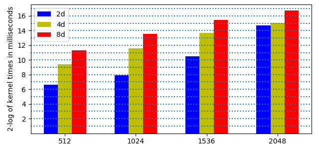
Fig. 141 2-logarithms of times on the V100 in 3 precisions.
Increasing precision, multipliers are 11.7 (2d to 4d) and 5.4 (4d to 8d), on 8 tiles for size 128, consider Fig. 142. The observed cost overhead factors are less than the multipliers. The heights of the bars in Fig. 142 follow a regular pattern.
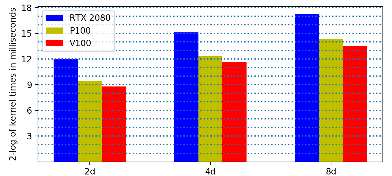
Fig. 142 2-logarithms of times on 3 GPUs in 3 precision.
Teraflop performance is attained at much lower dimensions for the QR than for the back substitution. A roofline plot is shown in Fig. 143 based on the data in Table 39.
\(n\) |
32 |
64 |
96 |
128 |
160 |
192 |
224 |
256 |
|---|---|---|---|---|---|---|---|---|
\((1)\) |
58.71 |
1500 |
2740 |
4308 |
6203 |
8427 |
10980 |
13860 |
\((2)\) |
119.1 |
263.9 |
440.7 |
633.8 |
679.0 |
852.9 |
1036.0 |
1113.6 |
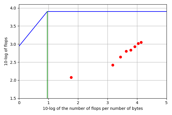
Fig. 143 Roofline plot for back substitution in quad double precision on the V100.
In a least squares solver, the back substitution is applied after the QR decomposition. In Table 40, timings are summarized for four precisions on the V100, for dimensions \(8 \times 128\). Teraflop performance is attained already in double double precision (2d).
stage BS after QR |
1d |
2d |
4d |
8d |
|---|---|---|---|---|
QR kernel time |
157.9 |
451.1 |
3020.6 |
11924.5 |
QR wall time |
204.0 |
566.0 |
3203.0 |
12244.0 |
BS kernel time |
2.0 |
4.0 |
28.0 |
114.5 |
BS wall time |
4.0 |
7.0 |
35.0 |
127.0 |
QR kernel flops |
303.4 |
2282.2 |
3369.8 |
4041.4 |
QR wall flops |
235.1 |
1819.6 |
3177.8 |
3936.1 |
BS kernel flops |
8.1 |
89.8 |
127.9 |
149.1 |
BS wall flops |
4.2 |
49.8 |
102.9 |
134.5 |
total kernel flops |
299.6 |
2262.9 |
3340.0 |
4004.4 |
total wall flops |
230.8 |
1797.3 |
3144.7 |
3897.0 |
Additional references and suggested references follow.
Bibliography
J. R. Shewchuk. Adaptive Precision Floating-Point Arithmetic and Fast Robust Geometric Predicates. Discrete & Computational Geometry 18, 305–363, 1997.
<https://docs.juliahub.com/MultiFloats>
MultiFloats.jlis a Julia package by David K. Zhang which outperforms theBigFloatmultiprecision arithmetic.N. Maho. MPLAPACK} version 2.0.1. user manual.
arXiv:2109.13406v2 [cs.MS] 12 Sep 2022. Offers support for quad double linear algebra operations and for arbitrary multiprecision linear system solvers.J.Verschelde. Least squares on GPUs in multiple double precision. In The 2022 IEEE International Parallel and Distributed Processing Symposium Workshops (IPDPSW), pages 828–837. IEEE, 2022.
Exercises
Provide a justification for the formulas in the WY representation: \(Q = Q + Q \star W \star Y^T\) and \(R = R + Y \star W^T \star C\).
Use the
MultiFloats.jlto build a multiple double version of the JuliahouseQRfunction.Describe a high level parallel Julia implementation by referring to the proper BLAS operations in the algorithm.