GPU Accelerated Newton’s Method for Taylor Series

The last application comes from computational algebra.

Problems Statement and Overview

Given is

1. a system of polynomials in several variables, where the coefficients are truncated power series in one variable; and

2. one vector of truncated power series as an approximate solution.

We assume that the problem is regular, that is: the series are Taylor series.

The difficulty of running Newton’s method is determined by

1. \(N\), the number of polynomials in the system;

2. \(n\), the number of variables in each polynomial;

3. \(d\), the degree of truncation of the series; and

4. \(\epsilon\), the working precision.

The main questions concerning the scalability are below.

1. What are the dimensions \((N, n, d, \epsilon)\) to fully occupy the GPU?

2. What is the cost of evaluation and differentiation on a GPU compared to the overall cost of one Newton step?

3. Can GPU acceleration compensate for the cost overhead caused by multiple double arithmetic? For which \(\epsilon\)?

Working with truncated power series, computing modulo \(O(t^d)\), is doing arithmetic over the field of formal series \({\mathbb C}[[t]]\). Linearization is applied: we consider \({\mathbb C}^n[[t]]\) instead of \({\mathbb C}[[t]]^n\). Instead of a vector of power series, we consider a power series with vectors as coefficients. What needs to be solved is \({\bf A} {\bf x} = {\bf b}\), \({\bf A} \in {\mathbb C}^{n \times n}[[t]]\), \({\bf b}, {\bf x} \in {\mathbb C}^n[[t]]\). For example:

\[\begin{split}\left[ \begin{array}{cccc} A_0 & & & \\ A_1 & A_0 & & \\ A_2 & A_1 & A_0 & \\ A_3 & A_2 & A_1 & A_0 \\ \end{array} \right] \left[ \begin{array}{c} {\bf x}_0 \\ {\bf x}_1 \\ {\bf x}_2 \\ {\bf x}_3 \end{array} \right] = \left[ \begin{array}{c} {\bf b}_0 \\ {\bf b}_1 \\ {\bf b}_2 \\ {\bf b}_3 \end{array} \right]\end{split}\]

linearizes \({\bf A}(t) {\bf x}(t) = {\bf b}(t)\), with

\[{\bf A}(t) = A_0 + A_1 t + A_2 t^2 + A_3 t^3,\]

\[{\bf x}(t) = {\bf x}_0 + {\bf x}_1 t + {\bf x}_2 t^2 + {\bf x}_3 t^3,\]

\[{\bf b}(t) = {\bf b}_0 + {\bf b}_1 t + {\bf b}_2 t^2 + {\bf b}_3 t^3.\]

Data Staging for Evaluation and Differentiation

The convolution

\[\left( x_0 + x_1 t + \cdots + x_d t^d \right) \star \left( y_0 + y_1 t + \cdots + y_d t^d \right)\]

has coefficients

\[z_k = \sum_{i=0}^k x_i \cdot y_{k-i}, \quad k = 0,1,\ldots,d.\]

In the accelerated version, thread \(k\) computes \(z_k\).

To avoid thread divergence, pad with zeros, e.g., for \(d=3\), consider Fig. 146.

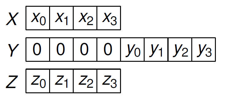
Fig. 146 Padding the second argument in a convolution with zeros introduces regularity: every thread performs the same number of operations.

The arrays \(X\), \(Y\), and \(Z\) shown in Fig. 146 are in shared memory. After loading the coefficients of the series into shared memory arrays, thread \(k\) computes

\[z_k = \sum_{i=0}^k x_i \cdot y_{k-i}, k = 0,1,\ldots,d.\]

Pseudo code is listed below:

1. \(X_k := x_k\)

2. \(Y_k := 0\)

3. \(Y_{d+k} := y_k\)

4. \(Z_k := X_0 \cdot Y_{d+k}\)

5. for \(i\) from 1 to \(d\) do \(Z_k := Z_k + X_i \cdot Y_{d+k-i}\)

6. \(z_k := Z_k\)

Evaluating and differentiating one monomial \(a~\!x_1 x_2 x_3 x_4 x_5\) at a power series vector:

\[\begin{split}\begin{array}{lll} f_1 := a \star z_1 & b_1 := z_5 \star z_4 \\ f_2 := f_1 \star z_2 % f_2 := a z_1 \star z_2 & b_2 := b_1 \star z_3 \\ % & b_2 := z_5 z_4 \star z_3 \\ f_3 := f_2 \star z_3 % f_3 := a z_1 z_2 \star z_3 & b_3 := b_2 \star z_2 % & b_3 := z_5 z_4 z_3 \star z_2 & c_1 := f_1 \star b_2 \\ % & c_1 := a z_1 \star z_5 z_4 z_3 \\ f_4 := f_3 \star z_4 % f_4 := a z_1 z_2 z_3 \star z_4 & b_3 := b_3 \star a % & b_3 := z_5 z_4 z_3 z_2 \star a & c_2 := f_2 \star b_1 \\ % & c_2 := a z_1 z_2 \star z_5 z_4 \\ f_5 := f_4 \star z_5 & % f_5 := a z_1 z_2 z_3 z_4 \star z_5 & & c_3 := f_3 \star z_5 % & c_3 := a z_1 z_2 z_3 \star z_5 \end{array}\end{split}\]

• The gradient is in \((b_3, c_1, c_2, c_3, f_4)\) and the value is in \(f_5\).

• Each \(\star\) is a convolution between two truncated power series.

• Statements on the same line can be computed in parallel.

Cost of accelerated monomial evaluation and differentation.

Given sufficiently many blocks of threads, monomial evaluation and differentiation takes \(n\) steps for \(n\) variables.

Consider then the accelerated algorithmic differentiation of one polynomial, as in the example below.

\[\begin{split}\begin{array}{rccccccc} p & = ~ a_0~+~ & a_1 x_1 x_3 x_6 & + & a_2 x_1 x_2 x_5 x_6 & + & a_3 x_2 x_3 x_4 \\ & & f_{1,1} := a_1 \star z_1 & & f_{2,1} := a_2 \star z_1 & & f_{3,1} := a_3 \star z_2 \\ & & f_{1,2} := f_{1,1} \star z_3 & & f_{2,2} := f_{2,1} \star z_2 & & f_{3,2} := f_{3,1} \star z_3 \\ & & f_{1,3} := f_{1,2} \star z_6 & & f_{2,3} := f_{2,2} \star z_5 & & f_{3,3} := f_{3,2} \star z_4 \\ & & & & f_{2,4} := f_{2,3} \star z_6 & & \\ & & b_{1,1} := z_6 \star z_3 & & b_{2,1} := z_6 \star z_5 & & b_{3,1} := z_4 \star z_3 \\ & & b_{1,1} := b_{1,1} \star a_1 & & b_{2,2} := b_{2,1} \star z_2 & & b_{3,1} := b_{3,1} \star a_3 \\ & & & & b_{2,2} := b_{2,2} \star a_2 & & \\ & & c_{1,1} := f_{1,1} \star z_6 & & c_{2,1} := f_{2,1} \star b_{2,1} & & c_{3,1} := f_{3,1} \star z_4 \\ & & & & c_{2,2} := f_{2,2} \star z_6 \end{array}\end{split}\]

The 21 convolutions are arranged below (on same line: parallel execution):

\[\begin{split}\begin{array}{ccccccccc} f_{1,1} & b_{1,1} & & f_{2,1} & b_{2,1} & & f_{3,1} & b_{3,1} \\ f_{1,2} & b_{1,1} & c_{1,1} & f_{2,2} & b_{2,2} & c_{2,1} & f_{3,2} & b_{3,1} & c_{3,1} \\ f_{1,3} & & & f_{2,3} & b_{2,2} & c_{2,2} & f_{3,3} & & \\ & & & f_{2,4} & & & & & \\ \end{array}\end{split}\]

For efficient computation, we must take care about the staging of the data.

For the example, the 21 convolutions

\[\begin{split}\begin{array}{ccccccccc} f_{1,1} & b_{1,1} & & f_{2,1} & b_{2,1} & & f_{3,1} & b_{3,1} \\ f_{1,2} & b_{1,1} & c_{1,1} & f_{2,2} & b_{2,2} & c_{2,1} & f_{3,2} & b_{3,1} & c_{3,1} \\ f_{1,3} & & & f_{2,3} & b_{2,2} & c_{2,2} & f_{3,3} & & \\ & & & f_{2,4} & & & & & \\ \end{array}\end{split}\]

are stored after the power series coefficients \(a_0\), \(a_1\), \(a_2\), \(a_3\), and the input power series \(z_1\), \(z_2\), \(z_3\), \(z_4\), \(z_5\), \(z_6\) in the array \(A\) in Fig. 147.

Fig. 147 One array \(A\) to stage all coefficients, values of the variables, the forward, backward, and cross values for the evaluation and the differentiation.

Observe in Fig. 147:

• The arrows point at the start position of the input series and at the forward \(f_{i,j}\), backward \(b_{i,j}\), cross products \(c_{i,j}\) for every monomial \(i\).

• For complex and multiple double numbers, there are multiple data arrays, for real, imaginary parts, and for each double in a multiple double.

One block of threads does one convolution.

It takes four kernel launches, to compute the 21 convolutions

\[\begin{split}\begin{array}{ccccccccc} f_{1,1} & b_{1,1} & & f_{2,1} & b_{2,1} & & f_{3,1} & b_{3,1} \\ f_{1,2} & b_{1,1} & c_{1,1} & f_{2,2} & b_{2,2} & c_{2,1} & f_{3,2} & b_{3,1} & c_{3,1} \\ f_{1,3} & & & f_{2,3} & b_{2,2} & c_{2,2} & f_{3,3} & & \\ & & & f_{2,4} & & & & & \\ \end{array}\end{split}\]

respectively with 6, 9, 5, and 1 block of threads.

Cost of accelerated convolutions for polynomial evaluation and differentiation.

Given sufficiently many blocks of threads, all convolutions for the polynomial evaluation and differentiation take \(m\) steps, where \(m\) is the largest number of variables in one monomial.

A convolution job \(j\) is defined by the triplet \((t_1(j), t_2(j), t_3(j))\), where

• \(t_1(j)\) and \(t_2(j)\) are the locations in the array \(A\) for the input, and

• \(t_3(j)\) is the location in \(A\) of the output of the convolution.

One block of threads does one addition of two power series. An addition job \(j\) is defined by the pair \((t_1(j), t_2(j))\), where

• \(t_1(j)\) is the location in the array \(A\) of the input, and

• \(t_2(j)\) is the location in the array \(A\) of the update.

Jobs are defined recursively, following the tree summation algorithm. The job index \(j\) corresponds to the block index in the kernel launch.

Cost of accelerated polynomial evaluation and differentiation

Given sufficiently many blocks of threads, polynomial evaluation and differentiation takes \(m + \lceil \log_2(N) \rceil\) steps, where \(m\) is the largest number of variables in one monomial and \(N\) is the number of monomials.

For \(N \gg m\), an upper bound for the speedup is \(d N/\log_2(N)\), where \(d\) is the degree at which the series are truncated.

The algorithmic differentiation was tested on five different GPUs. For the multiple double precision, code generated by the CAMPARY software, (by M. Joldes, J.-M. Muller, V. Popescu, W. Tucker, in ICMS 2016) was used on five different GPUs, with specifiation in Table 41

Table 41 specifications on five different GPUs.

NVIDIA GPU	CUDA	#MP	#cores/MP	#cores	GHz
Tesla C2050	2.0	14	32	448	1.15
Kepler K20C	3.5	13	192	2496	0.71
Pascal P100	6.0	56	64	3584	1.33
Volta V100	7.0	80	64	5120	1.91
GeForce RTX 2080	7.5	46	64	2944	1.10

The double peak performance of the P100 is 4.7 TFLOPS. At 7.9 TFLOPS, the V100 is 1.68 times faster than the P100. To evaluate the algorithms, compare the ratios of the wall clock times on the P100 over V100 with the factor 1.68.

Three polynomials \(p_1\), \(p_2\), and \(p_3\) were used for testing. For each polynomial:

• \(n\) is the total number of variables,

• \(m\) is the number of variables per monomial, and

• \(N\) is the number of monomials (not counting the constant term).

The last two columns of Table 42 list the number of convolution and addition jobs:

Table 42 characteristics of the test polynomials.

	n	m	N	#cnv	#add
\(p_1\)	16	4	1,820	16,380	9,084
\(p_2\)	128	64	128	24,192	8,192
\(p_3\)	128	2	8,128	24,256	24,256

Does the shape of the test polynomials influence the execution times?

In evaluating \(p_1\) for degree \(d = 152\) in deca double precision, the cudaEventElapsedTime measures the times of kernel launches. The last line is the wall clock time for all convolution and addition kernels. All units in Table 43 are milliseconds.

Table 43 performance of the first test polynomial.

	C2050	K20C	P100	V100	RTX 2080
convolution	12947.26	11290.22	1060.03	634.29	10002.32
addition	10.72	11.13	1.37	0.77	5.01
sum	12957.98	11301.35	1061.40	635.05	10007.34
wall clock	12964.00	11309.00	1066.00	640.00	10024.00

• The \(12964/640 \approx 20.26\) is for the V100 over the oldest C2050.

• Compare the ratio of the wall clock times for P100 over V100 \(1066/640 \approx 1.67\) with the ratios of theoretical double peak performance of the V100 of the P100: \(7.9/4.7 \approx 1.68\).

In 1.066 second, the P100 did 16,380 convolutions, 9,084 additions.

• One addition in deca double precision requires 139 additions and 258 subtractions of doubles, while one deca double multiplication requires 952 additions, 1743 subtractions, and 394 multiplications.

• One convolution on series truncated at degree \(d\) requires \((d+1)^2\) multiplications and \(d(d+1)\) additions.

• One addition of two series at degree \(d\) requires \(d+1\) additions.

So we have \(16,380 (d+1)^2\) multiplications and \(16,380 d(d+1) + 9,084(d+1)\) additions in deca double precision.

• One multiplication and one addition in deca double precision require respectively 3,089 and 397 double operations.

• The \(16,380 (d+1)^2\) evaluates to 1,184,444,368,380 and \(16,380 d(d+1) + 9,084(d+1)\) to 151,782,283,404 operations.

In total, in 1.066 second the P100 did 1,336,226,651,784 double float operations, reaching a performance of 1.25 TFLOPS.

To examine the scalability, consider

1. the doubling of the precision, in double, double double, quad double and octo double precision, for fixed degree 191; and

2. the doubling of the number of coefficients of the series, from 32 to 64, and from 64 to 128.

For increasing precision, the problem becomes more compute bound.

Wall clock times are shown in Fig. 148 to illustrate the cost of doubling the precision.

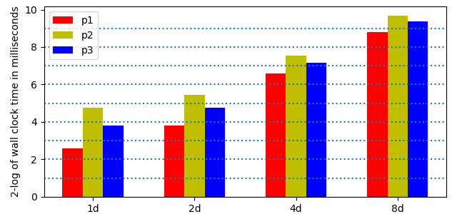
Fig. 148 The 2-logarithm of the wall clock times to evaluate and differentiate \(p_1\), \(p_2\), \(p_3\) in double (1d), double double (2d), quad double (4d), and octo double (8d) precision, for power series truncated at degree 191.

The effect of doubling the number of coefficients of the series is shown in Fig. 149.

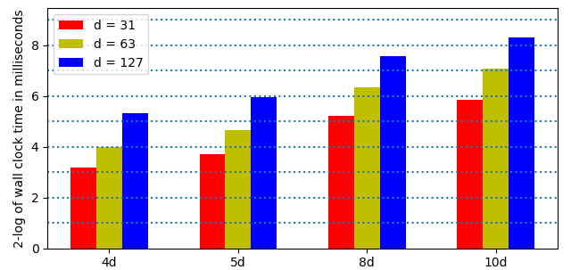
Fig. 149 The 2-logarithm of the wall clock times to evaluate and differentiate \(p_1\) in quad double (4d), penta double (5d), octo double (8d), and deca double (10d) precision, for power series of degrees 31, 63, and 127.

Accelerated Newton’s Method

To solve

\[\begin{split}\left[ \begin{array}{cccc} A_0 & & & \\ A_1 & A_0 & & \\ A_2 & A_1 & A_0 & \\ A_3 & A_2 & A_1 & A_0 \\ \end{array} \right] \left[ \begin{array}{c} {\bf x}_0 \\ {\bf x}_1 \\ {\bf x}_2 \\ {\bf x}_3 \end{array} \right] = \left[ \begin{array}{c} {\bf b}_0 \\ {\bf b}_1 \\ {\bf b}_2 \\ {\bf b}_3 \end{array} \right]\end{split}\]

in parallel, the task graph to solve a triangular block Toeplitz system is show in Fig. 150.

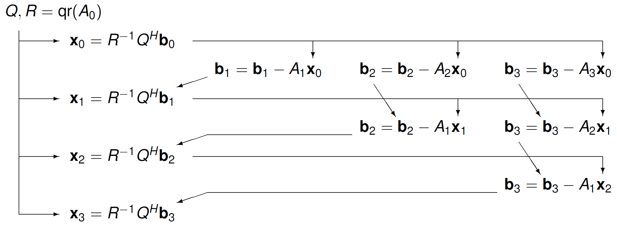
Fig. 150 A task graph for a triangular block Toeplitz system.

In the setup, we consider \(n\) variables \(\bf x\), an $n$-by-$n$ exponent matrix \(A\), and \({\bf b}(t)\) is a vector of \(n\) series of order \(O(t^d)\):

\[{\bf x}^A = {\bf b}(t) \quad \mbox{is a {\em monomial homotopy}.}\]

For example, \(n=3\), \({\bf x} = [x_1, x_2, x_3]\):

\[\begin{split}A = \left[ \begin{array}{ccc} 1 & 0 & 0 \\ 1 & 1 & 0 \\ 1 & 1 & 1 \end{array} \right] \quad \left\{ \begin{array}{lcl} x_1 & \!\!\!=\!\!\! & b_1(t) \\ x_1 x_2 & \!\!\!=\!\!\! & b_2(t) \\ x_1 x_2 x_3 & \!\!\!=\!\!\! & b_3(t) \end{array} \right. \quad \begin{array}{l} x_1(t) = \exp(\alpha_1 t) + O(t^d) \\ x_2(t) = \exp(\alpha_2 t) + O(t^d) \\ x_3(t) = \exp(\alpha_3 t) + O(t^d) \end{array}\end{split}\]

where

\[\exp(\alpha t) + O(t^4) = 1 + \alpha t + \frac{\alpha^2}{2!} t^2 + \frac{\alpha^3}{3!} t^3 + O(t^4),\]

with \(\alpha \in [-1, -1 + \delta] \cup [1 - \delta, 1]\), \(\delta > 0\), or \(|\alpha| = 1\) for random \(\alpha \in {\mathbb C}\).

To motivate the use of multiple double precision, consider the following series expansion:

\[\exp(t) = \sum_{k=0}^{d-1} \frac{t^k}{k!} + O(t^d)\]

In Table 44, the magnitude of the last coefficient is related to the required precision.

Table 44 Recommended precision for factorial coefficients.

\(k\)	\(1/k!\)	recommended precision
7	2.0e-004	double precision okay
15	7.7e-013	use double doubles
23	3.9e-023	use double doubles
31	1.2e-034	use quad doubles
47	3.9e-060	use octo doubles
63	5.0e-088	use octo doubles
95	9.7e-149	need hexa doubles
127	3.3e-214	need hexa doubles

The monomial homotopies allow to set the scalability parameters.

1. Going from one to two columns of monomials:

   \[{\bf c}_1 {\bf x}^{A_1} + {\bf c}_2 {\bf x}^{A_2} = {\bf b}(t),\]

   for two \(n\)-vectors \({\bf c}_1\) and \({\bf c}_2\) and two exponent matrices \(A_1\) and \(A_2\).

2. For increasing dimensions: \(n=64, 128, 256, 512, 1024\).

3. For increasing orders \(d\) in \(O(t^d)\), \(d = 1, 2, 4, 8, 16, 32, 64\).

4. For increasing precision: double, double double, quad double, octo double.

Doubling columns, dimensions, orders, and precision, how much of the overhead can be compensated by GPU acceleration?

This application combines different types of accelerated computations:

1. convolutions for evaluation and differentiation

2. Householder QR

3. \(Q^H {\bf b}\) computations

4. back substitutions to solve \(R {\bf x} = Q^H {\bf b}\)

5. updates \({\bf b} = {\bf b} - A {\bf x}\)

6. residual computations \(\| {\bf b} - A {\bf x} \|_1\)

Which of the six types occupies most time?

The computations are staggered. In computing \({\bf x}(t) = {\bf x}_0 + {\bf x}_1 t + {\bf x}_2 t^2 + \cdots + {\bf x}_{d-1} t^{d-1}\), observe:

1. Start \({bf x}_0\) with half its precision correct, otherwise Newton’s method may not converge.

2. Increase \(d\) in the order \(O(t^d)\) gradually, e.g.: the new \(d\) is \(d + 1 + d/2\), hoping (at best) for quadratic convergence.

3. Once \({\bf x}_k\) is correct, the corresponding \({\bf b}_k = 0\), as \({\bf b}_k\) is obtained by evaluation, and then the update \(\Delta {\bf x}_k\) should no longer be computed because

   \[QR \Delta {\bf x}_k = {\bf b}_k = {\bf 0} \quad \Rightarrow \quad \Delta {\bf x}_k = {\bf 0}.\]

This gives a criterion to stop the iterations.

To see which type of computation occupies the largest portion of the time, consider Fig. 151. and Fig. 152.

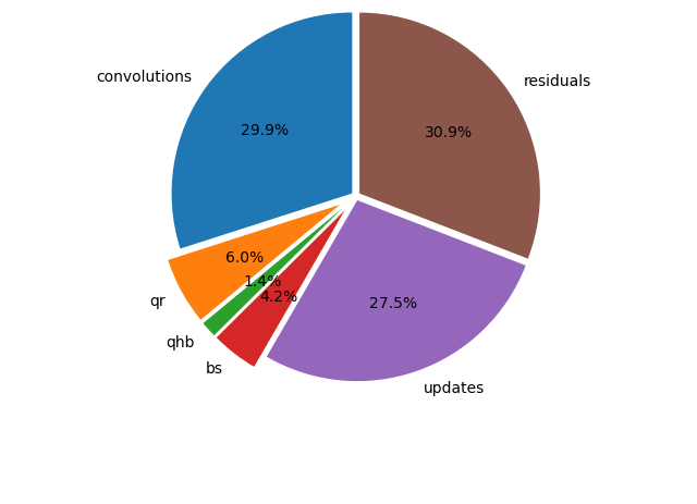
Fig. 151 Six different types of accelerated computations, on the V100, on one column of monomials, triangular exponent matrix of ones, \(n=1024\), \(d = 64\), 24 steps in octo double precision.

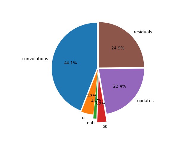
Fig. 152 Six different types of accelerated computations, on the V100, On two columns of monomials, triangular exponent matrix of ones, \(n=1024\), \(d = 64\), 24 steps in octo double precision.

Doubling the precision less than doubles the wall clock time and increases the time spent by all kernels, as illustrated by Fig. 153.

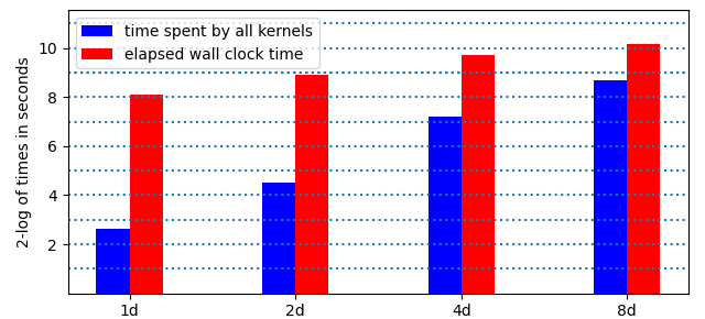
Fig. 153 On one column of monomials, triangular exponent matrix of ones, \(n=1024\), \(d=64\), 24 steps, 2-logarithms of times, in 4 different precisions, on the V100.

Teraflop performance of convolutions is illustrated in Fig. 154.

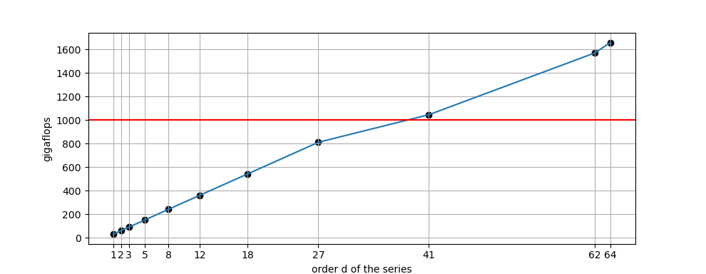
Fig. 154 On one column of monomials, triangular exponent matrix of ones, \(n=1024\), performance of the evaluation and differentiation, in octo double precision, for increasing orders of the series.

After degree 40, teraflop performance is observed on the V100.

Bibliography

• Accelerated polynomial evaluation and differentiation at power series in multiple double precision. In the 2021 IEEE International Parallel and Distributed Processing Symposium Workshops (IPDPSW), pages 740-749. IEEE, 2021. arXiv:2101.10881

• Least squares on GPUs in multiple double precision. In the 2022 IEEE International Parallel and Distributed Processing Symposium Workshops (IPDPSW), pages 828-837. IEEE, 2022. arXiv:2110.08375

• GPU Accelerated Newton for Taylor Series Solutions of Polynomial Homotopies in Multiple Double Precision. In the Proceedings of the 26th International Workshop on Computer Algebra in Scientific Computing (CASC 2024), pages 328-348. Springer, 2024. arXiv:2301.12659

The code at <https://github.com/janverschelde/PHCpack> is released under the GPL-3.0 License.