Parallel FFT and Isoefficiency

As our third application for parallel algorithms, we consider the Fast Fourier Transform (FFT). Instead of investigating the algorithmic aspects in detail, we introduce the FFT with an excellent software library FFTW which supports for OpenMP. The FFT is then used in the second part to illustrate the notion of isoefficiency, to complement the scalabiliy treatments in the laws of Ahmdahl and Gustafson.

The Fast Fourier Transform in Parallel

A periodic function \(f(t)\) can be written as a series of sinusoidal waveforms of various frequencies and amplitudes: the Fourier series. The Fourier transform maps \(f\) from the time to the frequency domain. In discrete form:

\[F_k = \frac{1}{n} \sum_{j=0}^{n-1} f_j e^{-2 \pi i (jk/n)}, \quad k=0,1,\ldots,n-1, f_k = f(x_k).\]

The Discrete Fourier Transform (DFT) maps a convolution into a componentwise product. The Fast Fourier Transform is an algorithm that reduces the cost of the DFT from \(O(n^2)\) to \(O(n \log(n))\), for length \(n\). The are many applications, for example: signal and image processing.

FFTW (the Fastest Fourier Transform in the West) is a library for the Discrete Fourier Transform (DFT), developed at MIT by Matteo Frigo and Steven G. Johnson available under the GNU GPL license at <http://www.fftw.org>. FFTW received the 1999 J. H. Wilkinson Prize for Numerical Software. FFTW 3.3.3 supports MPI and comes with multithreaded versions: with Cilk, Pthreads and OpenMP are supported. Before make install, do

./configure --enable-mpi --enable-openmp --enable-threads

We illustrate the use of FFTW for signal processing.

Consider \(f(t) = 2 \cos(4 \times 2 \pi t) + 5 \sin(10 \times 2 \pi t)\), for \(t \in [0,1]\). Its plot is in Fig. 30.

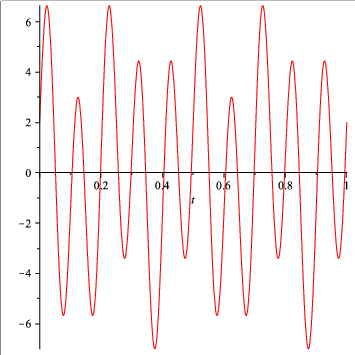
Fig. 30 A simple test signal.

Compiling and running the code below gives the frequencies and amplitudes of the test signal.

$ make fftw_use
gcc fftw_use.c -o /tmp/fftw_use -lfftw3 -lm
$ /tmp/fftw_use
scanning through the output of FFTW...
at 4 : (2.56000e+02,-9.63913e-14)
=> frequency 4 and amplitude 2.000e+00
at 10 : (-7.99482e-13,-6.40000e+02)
=> frequency 10 and amplitude 5.000e+00
$

Calling the FFTW software on a test signal:

#include <stdlib.h>
#include <stdio.h>
#include <math.h>
#include <fftw3.h>

double my_signal ( double t );
/*
 * Defines a signal composed of a cosine of frequency 4 and amplitude 2,
 * a sine of frequency 10 and amplitude 5. */

void sample_signal ( double f ( double t ), int m, double *x, double *y );
/*
 * Takes m = 2^k samples of the signal f, returns abscisses in x and samples in y. */

int main ( int argc, char *argv[] )
{
   const int n = 256;
   double *x, *y;
   x = (double*)calloc(n,sizeof(double));
   y = (double*)calloc(n,sizeof(double));
   sample_signal(my_signal,n,x,y);

   int m = n/2+1;
   fftw_complex *out;
   out = (fftw_complex*) fftw_malloc(sizeof(fftw_complex)*m);

   fftw_plan p;
   p = fftw_plan_dft_r2c_1d(n,y,out,FFTW_ESTIMATE);
   fftw_execute(p);
   printf("scanning through the output of FFTW...\n");
   double tol = 1.0e-8;  /* threshold on noise */
   int i;
   for(i=0; i<m; i++)
   {
      double v = fabs(out[i][0])/(m-1)
               + fabs(out[i][1])/(m-1);
      if(v > tol)
      {
         printf("at %d : (%.5e,%.5e)\n",
                i,out[i][0],out[i][1]);
         printf("=> frequency %d and amplitude %.3e\n",
                i,v);
      }
   }
   return 0;
}

running the OpenMP version of FFTW

For timing purposes, we define a program that takes in the parameters at the command line. The parameters are m and n: We will run the fftw m times for dimension n. The setup of our experiment is in the code below followed by the parallel version with OpenMP.

Setup of the experiment to execute the fftw:

#include <stdlib.h>
#include <stdio.h>
#include <time.h>
#include <math.h>
#include <fftw3.h>

void random_sequence ( int n, double *re, double *im );
/*
 * Returns a random sequence of n complex numbers
 * with real parts in re and imaginary parts in im. */

int main ( int argc, char *argv[] )
{
   int n,m;
   if(argc > 1)
      n = atoi(argv[1]);
   else
      printf("please provide dimension on command line\n");
   m = (argc > 2) ? atoi(argv[2]) : 1;
   double *x, *y;
   x = (double*)calloc(n,sizeof(double));
   y = (double*)calloc(n,sizeof(double));
   random_sequence(n,x,y);
   fftw_complex *in,*out;
   in = (fftw_complex*) fftw_malloc(sizeof(fftw_complex)*n);
   out = (fftw_complex*) fftw_malloc(sizeof(fftw_complex)*n);
   fftw_plan p;
   p = fftw_plan_dft_1d(n,in,out,FFTW_FORWARD,FFTW_ESTIMATE);
   clock_t tstart,tstop;
   tstart = clock();
   int i;
   for(i=0; i<m; i++) fftw_execute(p);
   tstop = clock();
   printf("%d iterations took %.3f seconds\n",m,(tstop-tstart)/((double) CLOCKS_PER_SEC));
   return 0;
}

Code to runt the OpenMP version of FFTW is below.

#include <omp.h>
#include <fftw3.h>

int main ( int argc, char *argv[] )
{
   int t;  /* number of threads */

   t = (argc > 3) ? atoi(argv[3]) : 1;

   int okay = fftw_init_threads();
   if(okay == 0)
      printf("error in thread initialization\n");
   omp_set_num_threads(t);
   fftw_plan_with_nthreads(t);

To define the compilation in the makefile, we must link with the OpenMP library version fftw3 and with the fftw3 library:

fftw_timing_omp:
        gcc -fopenmp fftw_timing_omp.c -o /tmp/fftw_timing_omp \
            -lfftw3_omp -lfftw3 -lm

Results are in Table 14 and Table 15.

Table 14 Running times (with the unix command time), for computing 1,000 DFTs for \(n = 100,000\), with p threads, where real = wall clock time, user = cpu time, sys = system time, obtained on two 8-core processors at 2.60 Ghz.

p	real	user	sys	speed up
1	2.443s	2.436s	0.004s	1
2	1.340s	2.655s	0.010s	1.823
4	0.774s	2.929s	0.008s	3.156
8	0.460s	3.593s	0.017s	5.311
16	0.290s	4.447s	0.023s	8.424

Table 15 Running times (with the unix command time), for computing 1,000 DFTs for \(n = 1,000,000\), with p threads, where real = wall clock time, user = cpu time, sys = system time, obtained on two 8-core processors at 2.60 Ghz.

p	real	user	sys	speed up
1	44.806s	44.700s	0.014s	1
2	22.151s	44.157s	0.020s	2.023
4	10.633s	42.336s	0.019s	4.214
8	6.998s	55.630s	0.036s	6.403
16	3.942s	62.250s	0.134s	11.366

Comparing the speedups in Table 14 with those in Table 15, we observe that speedups improve with a ten fold increase of \(n\). Next we introduce another way to think about scalability.

Isoefficiency

Before we examine how efficiency relates to scalability, recall some definitions. For p processors:

\[{\rm Speedup} = \frac{\rm serial~time}{\rm parallel~time} = S(p) \rightarrow p.\]

As we desire the speedup to reach p, the efficiency goes to 1:

\[{\rm Efficiency} = \frac{\rm Speedup}{p} = \frac{S(p)}{p} = E(p) \rightarrow 1.\]

Let \(T_s\) denote the serial time, \(T_p\) the parallel time, and \(T_0\) the overhead, then: \(p T_p = T_s + T_0\).

\[E(p) = \frac{T_s}{p T_p} = \frac{T_s}{T_s + T_0} = \frac{1}{1 + T_0/T_s}\]

The scalability analysis of a parallel algorithm measures its capacity to effectively utilize an increasing number of processors.

Let \(W\) be the problem size, for FFT: \(W = n \log(n)\). Let us then relate \(E\) to \(W\) and \(T_0\). The overhead \(T_0\) depends on \(W\) and \(p\): \(T_0 = T_0(W,p)\). The parallel time equals

\[T_p = \frac{W + T_0(W,p)}{p}, \quad \mbox{ Speedup } S(p) = \frac{W}{T_p} = \frac{W p}{W + T_0(W,p)}.\]

The efficiency

\[E(p) = \frac{S(p)}{p} = \frac{W}{W + T_0(W,p)} = \frac{1}{1 + T_0(W,p)/W}.\]

The goal is for \(E(p) \rightarrow 1$ as $p \rightarrow \infty\). The algorithm scales badly if W must grow exponentially to keep efficiency from dropping. If W needs to grow only moderately to keep the overhead in check, then the algorithm scales well.

Isoefficiency relates work to overhead:

\[\begin{split}\begin{array}{rcl} {\displaystyle E = \frac{1}{1 + T_0(W,p)/W}} & \Rightarrow & {\displaystyle \frac{1}{E} = \frac{1 + T_0(W,p)/W}{1}} \\ & \Rightarrow & {\displaystyle \frac{1}{E} - 1 = \frac{T_0(W,p)}{W}} \\ & \Rightarrow & {\displaystyle \frac{1-E}{E} = \frac{T_0(W,p)}{W}}. \end{array}\end{split}\]

The isoefficiency function is

\[W = \left( \frac{E}{1-E} \right) T_0(W,p) \quad {\rm or} \quad W = K ~\! T_0(W,p).\]

Keeping K constant, isoefficiency relates W to \(T_0\). We can relate isoefficiency to the laws we encountered earlier:

• Amdahl’s Law: keep W fixed and let p grow.
• Gustafson’s Law: keep p fixed and let W grow.

Let us apply the isoefficiency to the parallel FFT. The isoefficiency function: \(W = K~\! T_0(W,p)\). For FFT: \(T_s = n \log(n) t_c\), where \(t_c\) is the time for complex multiplication and adding a pair. Let \(t_s\) denote the startup cost and \(t_w\) denote the time to transfer a word. The time for a parallel FFT:

\[T_p = \underbrace{t_c \left( \frac{n}{p} \right) \log(n)}_{\mbox{computation time}} + \underbrace{t_s \log(p)}_{\mbox{start up time}} + \underbrace{t_w \left( \frac{n}{p} \right) \log(p)}_{\mbox{transfer time}}.\]

Comparing start up cost to computation cost, using the expression for \(T_p\) in the efficiency \(E(p)\):

\[\begin{split}\begin{array}{rcl} {\displaystyle E(p) = \frac{T_s}{p T_p}} & = & {\displaystyle \frac{n \log(n) t_c}{n \log(n) t_c + p \log(p) t_s + n \log(p) t_w}} \\ & = & {\displaystyle \frac{W t_c}{W t_c + p \log(p) t_s + n \log(p) t_w}, ~~ W = n \log(n)}. \end{array}\end{split}\]

Assume \(t_w = 0\) (shared memory):

\[E(p) = \frac{W t_c}{W t_c + p \log(p) t_s}.\]

We want to express \(\displaystyle K = \frac{E}{1-E}\), using \(\displaystyle \frac{1}{K} = \frac{1-E}{E} = \frac{1}{E} - 1\):

\[\frac{1}{K} = \frac{W t_c + p \log(p) t_s}{W t_c} - \frac{W t_c}{W t_c} \quad \Rightarrow \quad W = K \left( \frac{t_s}{t_c} \right) p \log(p).\]

The plot in Fig. 31 shows by how much the work load must increase to keep the same efficiency for an increasing number of processors.

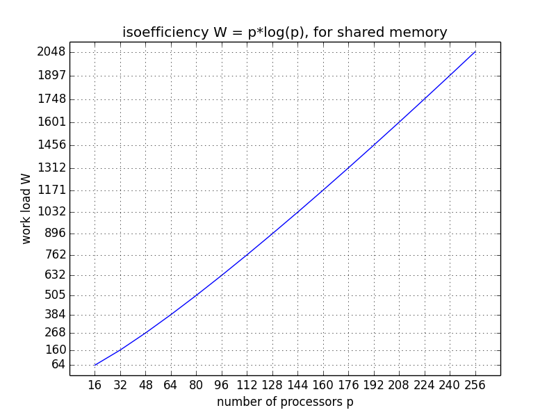
Fig. 31 Isoefficiency for a shared memory application.

Comparing transfer cost to the computation cost, taking another look at the efficiency \(E(p)\):

\[E(p) = \frac{W t_c}{W t_c + p \log(p) t_s + n \log(p) t_w}, \quad W = n \log(n).\]

Assuming \(t_s = 0\) (no start up):

\[E(p) = \frac{W t_c}{W t_c + n \log(p) t_w}.\]

We want to express \(\displaystyle K = \frac{E}{1-E}\), using \(\displaystyle \frac{1}{K} = \frac{1-E}{E} = \frac{1}{E} - 1\):

\[\frac{1}{K} = \frac{W t_c + n \log(p) t_w}{W t_c} - \frac{W t_c}{W t_c} \quad \Rightarrow \quad W = K \left( \frac{t_w}{t_c} \right) n \log(p).\]

In Fig. 32 the efficiency function is displayed for an increasing number of processors and various values of the dimension.

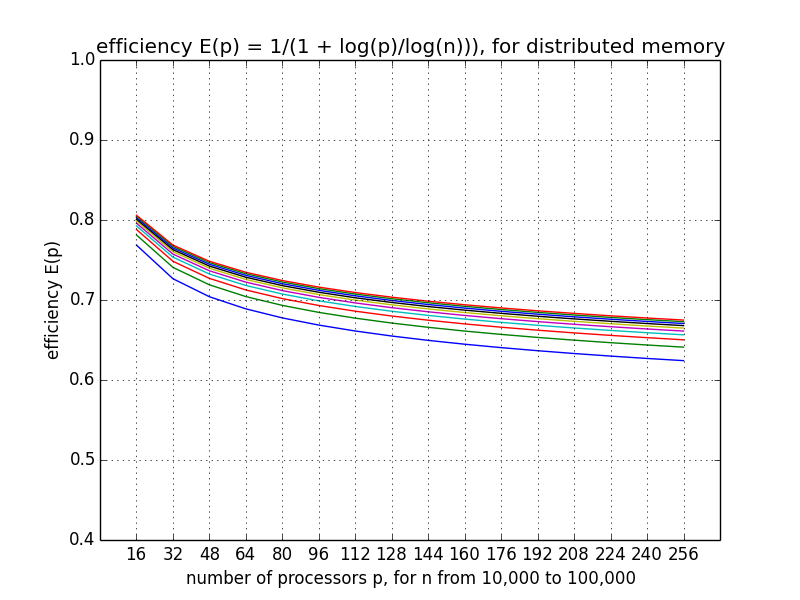
Fig. 32 Scalability analysis with a plot of the efficiency function.

Bibliography

1. Matteo Frigo and Steven G. Johnson: FFTW for version 3.3.3, 25 November 2012. Manual available at <http://www.fftw.org>.
2. Matteo Frigo and Steven G. Johnson: The Design and Implementation of FFTW3. Proc. IEEE 93(2): 216–231, 2005.
3. Vipin Kumar and Anshul Gupta: Analyzing Scalability of Parallel Algorithms and Architectures. Journal of Parallel and Distributed Computing 22: 379–391, 1994.
4. Ananth Grama, Anshul Gupta, George Karypis, Vipin Kumar: Introduction to Parallel Computing. 2nd edition, Pearson 2003. Chapter 13 is devoted to the Fast Fourier Transform.
5. Thomas Decker and Werner Krandick: On the Isoefficiency of the Parallel Descartes Method. In Symbolic Algebraic Methods and Verification Methods, pages 55–67, Springer 2001. Edited by G. Alefeld, J. Rohn, S. Rump, and T. Yamamoto.

Exercises

1. Investigate the speed up for the parallel FFTW with threads.
2. Consider the isoefficiency formulas we derived for a parallel version of the FFT. Suppose an efficiency of 0.6 is desired. For values \(t_c = 1\), \(t_s = 25\) and \(t_w = 4\), make plots of the speedup for increasing values of n, taking \(p=64\). Interpret the plots relating to the particular choices of the parameters \(t_c\), \(t_s\), \(t_w\), and the desired efficiency.
3. Relate the experimental speed ups with the theoretical isoefficiency formulas.