Options of the Executable phc
For many small to moderate size problems, the most convenient way to get an answer of phc is to call the blackbox solver with the option -b.
phc -0 : random numbers with fixed seed for repeatable runs
Many homotopy algorithms generate random constants. With each run, the current time is used to generate another seed for the random number generator, leading to different random constants in each run. As different random values give different random start systems, this may cause differences in the solution paths and fluctuations in the execution time. Another notable effect of generating a different random constant each time is that the order of the solutions in the list may differ. Although the same solutions should be found with each run, a solution that appears first in one run may turn out last in another run.
With the option -0, a fixed seed is used in each run. This option can be combined with the blackbox solver (phc -b), e.g.: phc -b -0 or phc -0 -b.
Since version 2.3.89, the option -0 is extended so the user may give the digits of the seed to be used. For example, calling phc as phc -089348224 will initialize the random number generator with the seed 89348224. Just calling phc as phc -0 will still result in using the same fixed seed as before in each run.
To reproduce a run with any seed (when the option -0 was not used), we can look at the output file, for the line
Seed used in random number generators : 407.
which appears at the end of the output of phc -b. Running phc -b -0407 on the same input file as before will generate the same sequences of random numbers and thus the same output.
A homotopy is a family of polynomial systems.
In an artificial parameter homotopy there is one parameter  usually going from 0 to 1.
If we want to solve the system
usually going from 0 to 1.
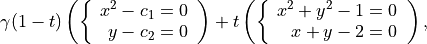
If we want to solve the system  and we have a system
  then a typical homotopy is
  as below.

The  is a complex constant on the unit circle
in the complex plane, generated uniformly at random.
If all solutions of are isolated
and of multiplicity one, then only for a finite number of complex values
for the homotopy has
singular solutions.
But since we consider
is a complex constant on the unit circle
in the complex plane, generated uniformly at random.
If all solutions of are isolated
and of multiplicity one, then only for a finite number of complex values
for the homotopy has
singular solutions.
But since we consider ![t \in [0,1]](_images/math/495cd8674616e3200753e6286e69a6d03f23effe.png) and since the values
for for which are complex,
the interval
and since the values
for for which are complex,
the interval  will with probability one not contain
any of the bad complex values for and therefore no
singular solutions for
will with probability one not contain
any of the bad complex values for and therefore no
singular solutions for  will occur.
Note that, for this gamma trick to work, the order of the operations matters.
We first give the program the system
and then either also give the system
or let the program generate a suitable .
Only then, in the construction of the homotopy will a random number
generator determine a constant .
If the is predetermined, then it is possible to
construct an input system and
a start system for which there
are bad values for .
But reverting the usual order of operations is a bit similar to guessing
the outcome of a coin toss after the coin toss and not before the coin toss.
Therefore phc -0 should be used only for debugging purposes.
phc -a : solving polynomial systems equation-by-equation
The equation-by-equation solver applies the diagonal homotopies to intersect the solution set of the current set of polynomials with the next polynomial equation. The user has the possibility to shuffle the order of input polynomials.
Consider for example the following system:
3
 (x-1)*(x^2 - y)*(x-0.5);
 (x-1)*(x^3 - z)*(y-0.5);
 (x-1)*(x*y - z)*(z-0.5);
Because of its factored form, we see that its solution set contains
at least one isolated point
 ;
;the twisted cubic
 ; and
; andthe two dimensional plane defined by
 .
.
The output of phc -a will produce three files,
with suffixes _w0, _w1, _w2, respectively
for the zero dimensional, the one dimensional,
and the two dimensional parts of the solution set.
a list of candidate isolated points;
generic points on the twisted cubic; and
one generic point on the plane
 .
.
The positive dimensional solution sets are each represented by a witness set. A witness set for a k-dimensional solution set of a system f consists of the system f, augmented with k linear equations with random coefficients, and solutions which satisfy the augmented system. Because the linear equations have random coefficients, each solution of the augmented system is a generic point. The number of generic points equals the degree of the solution set.
The output of phc -a gives a list of candidate witness points.
In the example, the list of candidate isolated points will most
likely contains points on higher dimensional solution sets.
Such points can be filtered away with the homotopy membership test
available in phc -f.
After filtering the points on higher dimensional solution sets,
each pure dimensional solution set may decompose in irreducible
components. The factorization methods of phc -f will partition
the witness points of a pure dimensional solution set according to
the irreducible factors.
The equation-by-equation solver gives bottom up way to compute
a numerical irreducible decomposition. The diagonal homotopies
can be called explicitly at each level with the option -c.
The alternative top down way is available in phc -c as well.
phc -b : batch or blackbox processing
As a simple example of the input format for phc -b,
consider the following three lines
2
 x**2 + 4*y**2 - 4;
        2*y**2 - x;
as the content of the file input.
See the section on phc -g for a description of the input format.
To run the blackbox solver at the command line,
type phc -b input output. The solutions of the system
are appended to the polynomials in the file input.
The file output also contains the solutions, in addition
to more diagnostics about the solving, such as the root counts,
start system, execution times.
The blackbox solver operates in four stages:
Preprocessing: scaling (
phc -s), handle special cases such as binomial systems.Counting the roots and constructing a start system (
phc -r). Various root counts, based on the degrees and Newton polytopes, are computed. The blackbox solver selects the smallest upper bound on the number of isolated solution in the computation of a start system to solve the given polynomial system.Track the solution paths from the solutions of the start system to the solutions of the target system (
phc -p).Verify whether all end points of the solution paths are distinct, apply Newton’s method with deflation on singular solutions (
phc -v).
Through the options -s, -r, -p, and -v,
the user can go through the stages separately.
See the documentation for phc -v for a description of the
quality indicators for the numerically computed solutions.
The blackbox solver recognizes several special cases:
one polynomial in one variable;
one system of linear equations;
a system with exactly two monomials in every equation.
For these special cases, no polynomial continuation is needed.
Polyhedral homotopies can solve Laurent systems,
systems where the exponents of the variables can be negative.
If the system on input is a Laurent system, then polyhedral
homotopies (see the documentation for -m) are applied directly
and no upper bounds based on the degrees are computed.
New since version 2.4.02 are the options -b2 and -b4 to run the
blackbox solver respectively in double double
and quad double precision,
for example as
phc -b2 cyclic7 c7out2
phc -b4 cyclic7 c7out4
The most computational intensive stage in the solver is in the
path tracking. Shared memory multitasked path trackers are
available in the path trackers for both the polyhedral homotopies to solve
a random coefficient system and for the
artificial-parameter homotopy towards the target system.
See the documentation for the option phc -t below.
When combining -b with -t (for example as phc -b -t4
to use 4 threads in the blackbox solver),
the m-homogeneous and linear-product degree bounds are not computed,
because the polyhedral homotopies are applied with pipelining,
interlacing the production of the mixed cells on one thread
with the solving of a random coefficient system with the other threads.
To run on all available cores, call as phc -b -t,
omitting the number of tasks.
The focus on -b is on isolated solutions.
For a numerical irreducible decomposition of all solutions,
including the positive dimensional ones, consider the options
-a, -c, and -f.
phc -B : numerical irreducible decomposition in blackbox mode
The -B option bundles the functionality of
phc -cto run a cascade homotopy to compute candidate generic points on all components of the solution set; andphc -fto filter the junk points (which are not generic points) and to factor pure dimensional solution sets into irreducible factors.
Since version 2.4.48, running phc -B provides
a complete numerical irreducible decomposition.
Consider for example the system
4
 (x1-1)*(x1-2)*(x1-3)*(x1-4);
 (x1-1)*(x2-1)*(x2-2)*(x2-3);
 (x1-1)*(x1-2)*(x3-1)*(x3-2);
 (x1-1)*(x2-1)*(x3-1)*(x4-1);
The system has 4 isolated solutions, 12 solution lines, one solution plane of dimension 2, and one solution plane of dimension 3. A numerical irreducible decomposition returns the 4 isolated solution points and one generic point on each of the 12 solution lines, one generic point on the 2-dimensional solution plane, and one generic point on the 3-dimensional solution plane.
phc -c : irreducible decomposition for solution components
In a numerical irreducible decomposition, positive dimensional solution sets are represented by a set of generic points that satisfy the given system and as many linear equations with random coefficients as the dimension of the solution set. The number of generic points in that so-called witness set then equals the degree of the solution set.
The menu structure for a numerical irreducible decomposition consists of three parts:
Running a cascade of homotopies to compute witness points.
Intersecting witness sets with diagonal homotopies.
For binomial systems, the irreducible decomposition yields lists of monomial maps.
For the cascade of homotopies, the first choice in the menu combines the next two ones. The user is prompted to enter the top dimension (which by default is the ambient dimension minus one) and then as many linear equations with random coefficients are added to the input system. In addition, as many slack variables are added as the top dimension. Each stage in the cascade removes one linear equation and solutions with nonzero slack variables at the start of the homotopy may end at solutions of lower dimension.
The classification of the witness points along irreducible factors
may happen with the third menu choice or, using different methods,
with phc -f. The third menu choice of phc -c applies
bivariate interpolation methods, while phc -f offers monodromy
breakup and a combinatorial factorization procedure.
The intersection of witness sets with diagonal homotopies
may be performed with extrinsic coordinates, which doubles
the total number of variables, or in an intrinsic fashion.
The intersection of witness sets is wrapped in phc -w.
The third block of menu options of phc -c concerns binomial systems.
Every polynomial equation in a binomial system has exactly two
monomials with a nonzero coefficient. The positive dimensional
solution sets of such a system can be represented by monomial maps.
For sparse polynomial systems,
monomial maps are much more efficient data structures than witness sets.
phc -d : linear and nonlinear reduction w.r.t. the total degree
Degree bounds for the number of isolated solution often overshoot the actual number of solution because of relationships between the coefficients. Consider for example the intersection of two circles. A simple linear reduction of the coefficient matrix gives an equivalent polynomial system (having the same number of affine solutions) but with lower degrees. Reducing polynomials to introduce more sparsity may also benefit polyhedral methods.
As an example, consider the intersection of two circles:
2
 x^2 + y^2 - 1;
 (x -  0.5)^2 + y^2 - 1;
A simple linear combination of the two polynomials gives:
2
 x^2 + y^2 - 1;
 x -  2.5E-1;
This reduced system has the same solutions, but only two instead of four solution paths need to be tracked.
Nonlinear reduction attempts to replace higher degree polynomials in the system by S-polynomials.
phc -e : SAGBI/Pieri/Littlewood-Richardson homotopies
Numerical Schubert calculus is the development of numerical homotopy algorithms to solve Schubert problems. A classical problem in Schubert calculus is the problem of four lines. Given four lines in three dimensional space, find all lines that meet the four given lines in a point. If the lines are in general position, then there are exactly two lines that satisfy the problem specification. Numerical homotopy continuation methods deform a given generic problem into special position, solve the problem in special position, and then deform the solutions from the special into the generic problem.
As Schubert calculus is a classical topic in algebraic geometry,
what seems less well known is that Schubert calculus offers a solution
to the output pole placement problem in linear systems control.
The option phc -k offers one particular interface dedicated to the
Pieri homotopies to solve the output pole placement problem.
A related problem that can be solved with Schubert calculus is the
completion of a matrix so that the completed matrix has a prescribed
set of eigenvalues.
In numerical Schubert calculus, we have three types of homotopies:
SAGBI homotopies solve hypersurface intersection conditions the extrinsic way. The problem is: in
 -space, where
  ,
for
,
for  given
given  -planes, compute all
 -planes which meet the -planes nontrivially.
Pieri homotopies are intrinsically geometric and are better able to solve more general problems in enumerate geometry. Pieri homotopies generalize SAGBI homotopies in two ways:
The intersection conditions may require that the planes meet in a space of a dimension higher than one. In addition to the
-planes, the intersection conditions
contain the dimensions of the spaces of intersection.The solutions may be curves that produce
-planes.
The problem may then be formulated as an interpolation problem.
Given are  interpolation points and as
many -planes on input. The solutions are curves of
degree
interpolation points and as
many -planes on input. The solutions are curves of
degree  that meet the given -planes at the
given interpolation points.
that meet the given -planes at the
given interpolation points.
Littlewood-Richardson homotopies solve general Schubert problems. On input is a sequence of square matrices. With each matrix corresponds a bracket of intersection conditions on
-planes. Each intersection condition is the dimension of
the intersection of a solution -plane with a linear space
with generators in one of the matrices in the sequence on input.
The earliest instances of SAGBI and Pieri homotopies were already available in version 2.0 of PHCpack. Since version 2.3.95, a more complete implementation of the Littlewood-Richardson homotopies is available.
phc -f : factor a pure dimensional solution set into irreducibles
The f in -f is the f of factor and filter.
The first basic filter allows for example to extract the real solutions from a given list. Other filtering criteria involve for example the residual, the estimate of the inverse condition numbers, and a test whether a coordinate of a solution is zero or not.
The second filter implements the homotopy membership test
to decide whether a point belongs to a witness set.
This filter is needed to process the superwitness sets
computed by phc -a or phc -c.
Given on input a witness set and a point,
this filter runs a homotopy to decide if the point belongs
to the positive dimensional solution set represented by
the given witness set.
The factorization method take on input a witness set for a pure dimensional solution set of a polynomial system. For small degrees, a combinatorial factorization method will be fast. The second factorization method applies monodromy loops, using the linear trace test as a stop criterion.
Another option in the menu of phc -f gives access to a
tropical method to detect a common factor of two Laurent polynomials.
phc -g : check the format of an input polynomial system
The purpose of phc -g is to check whether a given input
system has the right syntax. A related option is phc -o.
Use -g as phc -g input output where input and
output are the names of input and output files respectively.
If output is omitted, then the output can be written to screen.
If both input and output are omitted, then the user will
be prompted to provide the polynomials in the input system.
The input system can be a system of polynomials in several
variables with complex coefficients.
The first line on the input file must be the number of polynomials.
If the number of variables is different from the number of polynomials,
then the second number on the first line must be the number of variables.
Variables may have negative exponents, in which case the system
is recognized as a Laurent polynomial system.
Working with negative exponents can be useful to exclude solutions
with zero coordinates, as polyhedral homotopies (see phc -m)
are capable of avoiding to compute those type of solutions.
The division operator / may not appear in a monomial,
e.g.: x/y is invalid, but may be used in a coefficient,
such as in 5/7. While phc -g will parse 5/7 in
double precision, phc -v will use the proper extended
precision in its multiprecision root refinement.
The coefficients of the system will be parsed by phc -g as complex numbers
in double precision. There is also no need to declare variables,
the names of the variables will be added to the symbol table,
in the order of which they occur in the polynomials in the system.
A trick to impose an order on the variables is to start the first
polynomial with the zero polynomial, written as x - x + y - y,
to ensure that the symbol x comes prior to y.
Internally, the terms in a polynomial are ordered in a graded
lexicographical order.
Names that may not be used as names for variables are e, E
(because of the scientific format of floating-point numbers)
and i, I (because of the imaginary unit  ).
Every polynomial must be terminated by a semicolon, the
).
Every polynomial must be terminated by a semicolon, the ; symbol.
Starting the name of a variable with ; is in general a bad idea anyway,
but semicolons are used as terminating symbols in a polynomial.
Round brackets are for grouping the real and imaginary parts of
complex coefficients, e.g.: (1.e-3 + 3/7*I)*x^2*y
or for grouping factors, e.g.: 3.14*(x+y)*(x-1)^4.
phc -h : writes helpful information to screen
The information written by phc -h is the condensed version
of this document. For every option, some helpful information
is defined. For example, typing phc -z -h or phc -h -z
displays information about phc -z.
Typing phc -h -h displays the list of all available options.
Instead of -h, one can also type --help.
phc -j : path tracking with algorithmic differentiation
In the tracking of a solution path we frequently apply Newton’s method. To run Newton’s method we need to evaluate the system and compute all its partial derivatives. The cost of evaluation and differentiation is a significant factor in the total cost. For large systems, this cost may even dominate.
The phc -j gives access to the Path library developed to
accelerate the path trackers with graphics processing units.
The code is capable to evaluate and differentiate large polynomial
systems efficiently, in double, double double, and quad double precision.
phc -k : realization of dynamic output feedback placing poles
The homotopies in numerical Schubert calculus (see the option -e)
solve the output pole placement problem in linear systems control.
The option -k applies the Pieri homotopies to compute feedback laws
for plants defined by (A,B,C) matrices.
For examples of input, see the Feedback/Data folder of the source code.
The feedback laws in the output file are realized and written
in a format ready for parsing with MATLAB or Octave.
The computation of output feedback laws is an application
of the Pieri homotopies, available via phc -e.
phc -l : witness set for hypersurface cutting with random line
A hypersurface defined by a polynomial in several variables is cut with one general line. The number of points on the hypersurface and the general line equal the degree of the hypersurface. This collection of points on the intersection of a hypersurface and a general line form a witness set.
For example, if the file sphere contains
1 3
x^2 + y^2 + z^2 - 1;
then typing at the command prompt
phc -l sphere sphere.out
results in the creation of the file sphere_w2 which contains
a witness set of dimension two for the unit sphere.
The output file sphere.out contains diagnostics about the computation.
For hypersurfaces of higher degree, the double precision as provided
by the hardware may turn out to be insufficient to compute as many
generic points as the degree of the hypersurface.
Therefore, the options l2 and l4 perform the computations
respectively in double double and quad double precision.
To continue the example from above, typing at the command prompt
phc -l4 sphere sphere.qd
will give two generic points on the sphere, computed in quad double precision.
phc -m : mixed volumes, MixedVol, DEMiCs, polyhedral homotopies
The menu choices of phc -m are a subset of the menu of phc -r.
The focus on phc -m is on mixed volumes. For polynomial systems
with as many equations as unknowns, the mixed volume of the Newton
polytopes gives a generically sharp upper bound on the number of
isolated solutions with coordinates different from zero.
The ability to focus only on solutions with all coordinates different from zero stems from the fact that shifting Newton polytopes (which corresponds to multiplying the polynomials with one monomial) does not increase their volumes. With polyhedral homotopies, we can solve systems of polynomials with negative exponents for the variables, the so-called Laurent polynomials.
The mixed volume of a tuple of Newton polytopes is defined as the coefficient in the expansion of the volume of a linear combination of Newton polytopes. For example, for a 3-tuple of Newton polytopes:
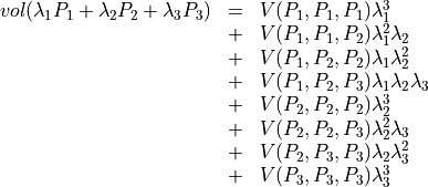
where  is the volume function
and
is the volume function
and  is the mixed volume.
For the tuple
is the mixed volume.
For the tuple  , its mixed volume
is
, its mixed volume
is  in the expansion above.
The polynomial above can be called the Minkowski polynomial and with the Cayley trick we can compute all its coefficients. This is implemented with the dynamic lifting algorithm.
The menu with 6 different lifting strategies is displayed as follows:
MENU with available Lifting Strategies (0 is default) :
  0. Static lifting     : lift points and prune lower hull.
  1. Implicit lifting   : based on recursive formula.
  2. Dynamic lifting    : incrementally add the points.
  3. Symmetric lifting  : points in same orbit get same lifting.
  4. MixedVol Algorithm : a faster mixed volume computation.
  5. DEMiCs Algorithm   : dynamic enumeration for mixed cells.
The menu of phc -m offers 5 different algorithms:
Static lifting: a lifting function is applied to the points in the support sets of the polynomials in the system and the lower hull defines the mixed cells. The users can specify the lifting values interactively. Liftings that do not lead to cells that are fine mixed are subdivided with a random lifting.
Implicit lifting: based on a recursive formula used in Bernshtein’s original proof that the mixed volumes bounds the number of isolated solutions with nonzero coordinates.
Dynamic lifting: points are added one after the other in an incremental construction of a mixed cell configuration. An implementation of the Cayley trick gives the Minkowski polynomial.
Symmetric lifting: many systems have Newton polytopes that are invariant to permutation symmetry. Even if the original system is not symmetric, the construction of the start system could benefit from the exploitation of this permutation symmetry.
The MixedVol Algorithm is a specific implementation of the static lifting method, applying a floating random lifting function.
The code offered with this option is a translation of software described in the paper by Tangan Gao, T. Y. Li, Mengnien Wu: Algorithm 846: MixedVol: a software package for mixed-volume computation. ACM Transactions on Mathematical Software, 31(4):555-560, 2005; distributed under the terms of the GNU General Public License as published by the Free Software Foundation.
With the stable mixed volume we count all affine solutions (not only those with nonzero coordinates) and then and obtain polyhedral homotopies that compute all affine solutions.
The DEMiCs Algorithm is faster than MixedVol for larger polynomial systems with many different supports. The algorithm is described in the paper by T. Mizutani, A. Takeda, and M. Kojima: Dynamic enumeration of all mixed cells, published in Discrete Comput. Geom. 37(3):351-367, 2007. The software DEMiCs is distributed under the GNU GPL license as well.
On multicore computers,
the solution of a random coefficient system
with polyhedral homotopies runs in parallel when calling phc with
the option -t. For example, phc -m -t8 will run the
polyhedral path trackers with 8 tasks.
To run on all available cores, call as phc -m -t,
omitting the number of tasks.
Since version 2.4.06,
the mixed volume computation by the MixedVol algorithm
(option 4 of phc -m) is interlaced with the path tracking
in a heterogenous pipelined application of multitasking.
phc -o : writes the symbol table of an input system
Running phc -o with as input argument a polynomial system
writes the symbols for the variables in the order in which they
are stored internally after parsing the system.
For example, if the file /tmp/ex1 contains the lines
2
  y + x + 1;
  x*y - 1;
then running phc -o at the command prompt as
phc -o /tmp/ex1 /tmp/ex1.out
makes the file /tmp/ex1.out which contains the line
y x
because in the formulation of the polynomial system,
the variable with name y occurred before the variable with name x.
Consequently, the order of the coordinates of the solutions will
then also be stored in the same order as of the occurrence of the
variable names.
If a particular order of variables would be inconvenient,
then a trick to force an order on the variables is to insert
a simple polynomial that simplifies to zero. For example,
a modification of the file /tmp/ex1 could be
2
 x + y - x - y +
 y + x + 1;
 x*y - 1;
and the first four monomials x + y - x - y will initialize the
symbol table with the names x and y, in that order.
phc -p : polynomial continuation in one parameter
We distinguish between two types of homotopies.
In an artificial parameter homotopy, the user is
prompted for a target system and a start system with start solutions.
If the input to phc -p is a polynomial system with one more unknown
than the number of equations,
then we have a natural parameter homotopy and the user
is then prompted to define one unknown as the continuation parameter.
We first illustrate artificial parameter homotopy continuation.
In the example below, the artificial parameter is denoted
by and, as goes from zero to one,
a simpler polynomial system, the start system, is deformed
to the target system, the system we want to solve:
where ,  , and
, and  are constants,
generated at random on the unit circle in the complex plane.
are constants,
generated at random on the unit circle in the complex plane.
For this example, the file with the target system contains
2
 x^2 + y^2 - 1;
 x + y - 2;
and the start system is then stored in the file with contents
2
 x^2 +(-7.43124688174374E-01 - 6.69152970422862E-01*i);
 y +(-7.98423708079157E-01 + 6.02095990999051E-01*i);

THE SOLUTIONS :
2 2
===========================================================================
solution 1 :
t :  0.00000000000000E+00   0.00000000000000E+00
m : 1
the solution for t :
 x : -9.33575033988799E-01  -3.58381997194074E-01
 y :  7.98423708079157E-01  -6.02095990999051E-01
== err :  0.000E+00 = rco :  1.000E+00 = res :  0.000E+00 ==
solution 2 :
t :  0.00000000000000E+00   0.00000000000000E+00
m : 1
the solution for t :
 x :  9.33575033988799E-01   3.58381997194074E-01
 y :  7.98423708079157E-01  -6.02095990999051E-01
== err :  0.000E+00 = rco :  1.000E+00 = res :  0.000E+00 ==
The start system can be constructed with phc -r.
With phc -p, the user has full access to all numerical tolerances
that define how close the numerical approximations have to stay
along a solution path. By default, path tracking happens in double
precision, but the user can increase the precision via the menu of
the homotopy settings.
At the command line, launching phc with the options -p2
and -p4 will run the path tracking respectively in double double
and quad double precision.
To rerun a selection of solution paths, the user should submit a start
system which contains only the start solutions of those paths that need
to be recomputed. In a rerun, one must choose the same
as in the previous run.
In addition to the artificial parameter increment-and-fix continuation, there is support for complex parameter continuation and real pseudo arc length path tracking with detection of singularities using the determinant of the Jacobian along the solution path.
To run pseudo arc length continuation, the user has to submit a system that has fewer equations than variables. For example, for a real sweep of the unit circle, the input would be
2 3
 x^2 + y^2 - 1;
 y*(1-s) + (y-2)*s;
where the last equation moves the line  to
to  .
The sweep will stop at the first singularity it encounters on the
solution path, which in this case is the
quadratic turning point at
.
The sweep will stop at the first singularity it encounters on the
solution path, which in this case is the
quadratic turning point at  .
.
The corresponding list of solutions should then contain the following:
2 3
===========================================================================
solution 1 :
t :  0.00000000000000E+00   0.00000000000000E+00
m : 1
the solution for t :
 x : -1.00000000000000E+00   0.00000000000000E+00
 y :  0.00000000000000E+00   0.00000000000000E+00
 s :  0.00000000000000E+00   0.00000000000000E+00
== err :  0.000E+00 = rco :  1.863E-01 = res :  0.000E+00 ==
solution 2 :
t :  0.00000000000000E+00   0.00000000000000E+00
m : 1
the solution for t :
 x :  1.00000000000000E+00   0.00000000000000E+00
 y :  0.00000000000000E+00   0.00000000000000E+00
 s :  0.00000000000000E+00   0.00000000000000E+00
== err :  0.000E+00 = rco :  1.863E-01 = res :  0.000E+00 ==
After launching the program as phc -p the user can determine the
working precision. This happens differently for the two types of
homotopies, depending on whether the parameter is natural or artificial:
For a natural parameter homotopy like the sweep, the user will be prompted explicitly to choose between double, double double, or quad double precision.
For an artificial parameter homotopy, the user can determine the working precision at the construction of the homotopy.
In both types of homotopies, natural parameter and aritificial parameter,
the user can preset the working precision respectively to double double
or quad double, calling the program as phc -p2 or as phc -p4.
Since version 2.4.13, phc -p provides path tracking for
overdetermined homotopies, where both target and start system
are given as overconstrained systems and every convex linear
combination between target and start system admits solutions.
phc -q : tracking solution paths with incremental read/write
For huge polynomial systems, all solutions may not fit in memory. The jumpstarting method for a polynomial homotopy does not require the computation of all solutions of the start system and neither does it keep the complete solution list in memory.
The phc -q is a byproduct of the distributed memory parallel
path trackers with developed with the Message Passing Interface (MPI).
Even if one is not concerned about memory use, phc -q is an
example of program inversion. Instead of first completely solving
the start system before tracking solution paths to the target system,
one can ask for the next start solution whenever one wants to compute
another solution of the target system.
The menu of types of supported homotopies is
MENU for type of start system or homotopy :
  1. start system is based on total degree;
  2. a linear-product start system will be given;
  3. start system and start solutions are provided;
  4. polyhedral continuation on a generic system;
  5. diagonal homotopy to intersect algebraic sets;
  6. descend one level down in a cascade of homotopies;
  7. remove last slack variable in a witness set.
The first four options concern isolated solutions of polynomial systems.
To construct a start system based on total degree
or a linear-product start system, use phc -r.
The polyhedral continuation needs a mixed cell configuration,
which can be computed with phc -m.
Options 5 and 6 deal with positive dimensional solution sets,
see phc -c.
phc -r : root counting and construction of start systems
The root count determines the number of solution paths that are tracked in a homotopy connecting the input system with the start system that has as many solutions as the root count. We have an optimal homotopy to solve a given system if the number of solution paths equals the number of solutions of the system.
Methods to bound the number of isolated solutions of a polynomial system fall in two classes:
Bounds based on the highest degrees of polynomials and variable groupings.
Bounds based on the Newton polytopes of the polynomials in the system. See the documentation for
phc -m.
The complete menu (called with cyclic 5-roots, with total degree 120) is shown below:
MENU with ROOT COUNTS and Methods to Construct START SYSTEMS :
  0. exit - current root count is based on total degree : 120
PRODUCT HOMOTOPIES based on DEGREES ------------------------------
  1. multi-homogeneous Bezout number               (one partition)
  2. partitioned linear-product Bezout number    (many partitions)
  3. general linear-product Bezout number          (set structure)
  4. symmetric general linear-product Bezout number (group action)
POLYHEDRAL HOMOTOPIES based on NEWTON POLYTOPES ------------------
  5. combination between Bezout and BKK Bound   (implicit lifting)
  6. mixed-volume computation                     (static lifting)
  7. incremental mixed-volume computation        (dynamic lifting)
  8. symmetric mixed-volume computation        (symmetric lifting)
  9. using MixedVol Algorithm to compute the mixed volume fast (!)
At the start, the current root count is the total degree,
which is the product of the degrees of the polynomials in the system.
The options 5 to 9 of the menu are also available in phc -m.
Three different generalizations of the total degree are available:
For a multi-homogeneous Bezout number, we split the set of variables into a partition. A classical example is the eigenvalue problem. When viewed as a polynomial system
 we see quadratic equations. Separating the variable for the
eigenvalue
we see quadratic equations. Separating the variable for the
eigenvalue  from the coordinates
  of
the eigenvectors turns the system into a multilinear problem
and provides the correct root count.
of
the eigenvectors turns the system into a multilinear problem
and provides the correct root count.In a partitioned linear-product Bezout number, we allow that the different partitions of the sets of variables are used for different polynomials in the system. This may lead to a lower upper bound than the multi-homogeneous Bezout number.
A general linear-product Bezout number groups the variables in a collection of sets where each variable occurs at most once in each set. Every set then corresponds to one linear equation. The formal root count is a generalized permanent, computed formally via algorithms for the bipartite matching problem.
Each of these three generalizations leads to a linear-product start system. Every start solution is the solution of a linear system. One can view the construction of a linear-product start system as the degeneration of the given polynomial system on input such that every input polynomial is degenerated to a product of linear factors.
The fourth option of the -r allows one to take
permutation symmetry
into account to construct symmetric start systems.
If the start system respects the same permutation symmetry as the
system on input, then one must track only those paths starting at
the generators of the set of start solutions.
After the selection of the type of start system, the user has the
option to delay the calculation of all start solutions.
All start solutions can be computed at the time when needed by phc -q.
To use the start system with phc -p, the user must ask to compute
all start solutions with -r.
phc -s : equation and variable scaling on system and solutions
A system is badly scaled if the difference in magnitude between the coefficients is large. In a badly scaled system we observe very small and very large coefficients, often in the same polynomial. The solutions in a badly scaled system are ill conditioned: small changes in the input coefficients may lead to huge changes in the coordinates of the solutions.
Scaling is a form of preconditioning. Before we solve the system, we attempt to reformulate the original problem into a better scaled one. We distinguish two types of scaling:
equation scaling: multiply every coefficient in the same equation by the same constant; and
variable scaling: multiply variables by constants.
Chapter 5 of the book of Alexander Morgan on Solving Polynomial Systems Using Continuation for Engineering and Scientific Problems (volume 57 in the SIAM Classics in Applied Mathematics, 2009) describes the setup of an optimization problem to compute coordinate transformations that lead to better values of the coefficients.
If the file /tmp/example contains the following lines
2
 0.000001*x^2 + 0.000004*y^2 - 4;
 0.000002*y^2 - 0.001*x;
then a session with phc -s (at the command prompt)
to scale the system goes as follows.
$ phc -s
Welcome to PHC (Polynomial Homotopy Continuation) v2.3.99 31 Jul 2015
Equation/variable Scaling on polynomial system and solution list.

MENU for the precision of the scalers :
  0. standard double precision;
  1. double double precision;
  2. quad double precision.
Type 0, 1, or 2 to select the precision : 0

Is the system on a file ? (y/n/i=info) y

Reading the name of the input file.
Give a string of characters : /tmp/example

Reading the name of the output file.
Give a string of characters : /tmp/example.out

MENU for Scaling Polynomial Systems :
  1 : Equation Scaling : divide by average coefficient
  2 : Variable Scaling : change of variables, as z = (2^c)*x
  3 : Solution Scaling : back to original coordinates
Type 1, 2, or 3 to select scaling, or i for info : 2
  Reducing the variability of coefficients ? (y/n) y
  The inverse condition is  4.029E-02.

Do you want the scaled system on separate file ? (y/n) y
Reading the name of the output file.
Give a string of characters : /tmp/scaled

$
Then the contents of the file /tmp/scaled is
2
x^2+ 9.99999999999998E-01*y^2-1.00000000000000E+00;
y^2-1.00000000000000E+00*x;

SCALING COEFFICIENTS :

10
3.30102999566398E+00   0.00000000000000E+00
3.00000000000000E+00   0.00000000000000E+00
-6.02059991327962E-01   0.00000000000000E+00
-3.01029995663981E-01   0.00000000000000E+00
We see that the coefficients of the scaled system are much nicer
than the coefficients of the original problem.
The scaling coefficients are needed to transform the solutions
of the scaled system into the coordinates of the original problem.
To transform the solutions, choose the third option of the second
menu of phc -s.
phc -t : tasking for tracking paths using multiple threads
The problem of tracking a number of solution paths can be viewed as a pleasingly parallel problem, because the paths can be tracked independently from each other.
The option -t allows the user to take advantage
of multicore processors.
For example, typing at the command prompt.
phc -b -t4 cyclic7 /tmp/cyclic7.out
makes that the blackbox solver uses 4 threads to solve the system.
If there are at least 4 computational cores available,
then the solver may finish its computations up to 4 times faster
than a sequential run.
To run on all available cores, call as phc -b -t,
omitting the number of tasks.
With the time command, we can compare the wall clock time between a sequential run and a run with 16 tasks:
time phc -b cyclic7 /tmp/cyc7t1

real    0m10.256s
user    0m10.202s
sys     0m0.009s

time phc -b -t16 cyclic7 /tmp/cyc7t16

real    0m0.851s
user    0m11.149s
sys     0m0.009s
The speedup on the wall clock time is about 12, obtained as 10.256/0.851.
The relationship with double double and quad double precision is interesting, consider the following sequence of runs:
time phc -b cyclic7 /tmp/c7out1

real    0m9.337s
user    0m9.292s
sys     0m0.014s

time phc -b -t16 cyclic7 /tmp/c7out2

real    0m0.923s
user    0m13.034s
sys     0m0.010s
With 16 tasks we get about a tenfold speedup, but what if we ask to double the precision?
time phc -b2 -t16 cyclic7 /tmp/c7out3

real    0m4.107s
user    0m59.164s
sys     0m0.018s
We see that with 16 tasks in double precision, the elapsed time equals 4.107 seconds, whereas the time without tasking was 9.337 seconds. This means that with 16 tasks, for this example, we can double the working precision and still finish the computation is less than half of the time without tasking. We call this quality up.
For quad double precision, more than 16 tasks are needed to offset the overhead caused by the quad double arithmetic:
time phc -b4 -t16 cyclic7 /tmp/c7out4

real    0m53.865s
user    11m56.630s
sys     0m0.248s
To track solution paths in parallel with phc -p,
for example with 4 threads, one needs to add -t4 to the
command line and call phc as phc -p -t4.
The option -t can also be added to phc -m at the command line,
to solve random coefficient start systems with polyhedral homotopies
with multiple tasks.
phc -u : Newton’s method and continuation with power series
The application of Newton’s method over the field of truncated power
series in double, double double, or quad double precision,
can be done with phc -u.
On input is a polynomial system where one of the variables will
be considered as a parameter in the series.
The other input to phc -u is a list of solution for the zero
value of the series variable.
Consider for example the intersection of the Viviani curve with a plane, as defined in the homotopy:
3 4
 (1-s)*y + s*(y-1);
 x^2 + y^2 + z^2 - 4;
 (x-1)^2 + y^2 - 1;
At s=0, the point (0,0,2) is a regular solution
and the file with the homotopy should contain
solution 1 :
t :  1.00000000000000E+00   0.00000000000000E+00
m : 1
the solution for t :
 s :  0.00000000000000E+00   0.00000000000000E+00
 y :  0.00000000000000E+00   0.00000000000000E+00
 x :  0.00000000000000E+00   0.00000000000000E+00
 z :  2.00000000000000E+00   0.00000000000000E+00
== err :  0.000E+00 = rco :  3.186E-01 = res :  0.000E+00 ==
The input file can be prepared inserting the s=0 into the homotopy
and giving to the blackbox solver phc -b a file with contents:
4
 s;
 (1-s)*y + s*(y-1);
 x^2 + y^2 + z^2 - 4;
 (x-1)^2 + y^2 - 1;
The output of phc -b will have the point (0,0,2) for s=0.
phc -v : verification, refinement and purification of solutions
While solution paths do in general not become singular or diverge, at the end of the paths, solutions may turn out to be singular and/or at infinity.
Consider for example the system
2
 x*y + x - 0.333;
 x^2 + y - 1000;
where the first solution obtained by some run with phc -b is
solution 1 :
t :  1.00000000000000E+00   0.00000000000000E+00
m : 1
the solution for t :
 x :  3.32667332704111E-04  -2.78531008415435E-26
 y :  9.99999999889332E+02   0.00000000000000E+00
== err :  3.374E-09 = rco :  2.326E-06 = res :  3.613E-16 ==
The last three numbers labeled with err, rco, and res
are indicators for the quality of the solution:
err: the magnitude of the last correction made by Newton’s method to the approximate solution. Theerrmeasures the forward error on the solution. The forward error is the magnitude of the correction we have to make to the approximate solution to obtain the exact solution. As the value oferris about1.0e-9we can hope to have about eight correct decimal places in the solution.rco: an estimate for the inverse of the condition number of the Jacobian matrix at the approximation for the solution. A condition number measures by how much a solution may change as by a change on the input coefficients. In the example above, the0.333could be a three digit approximation for1/3, so the error on the input could be as large as1.0e-4. Asrcois about1.0e-6, the condition number is estimated to be of order1.0e+6. For this example, an error of on the input coefficients
can result in an error of
on the input coefficients
can result in an error of  on the solutions.
res: the magnitude of the polynomials in the system evaluated at the approximate solution, the so-called residual. For this problem, the residual is the backward error. Because of numerical representation errors, we have not solved an exact problem, but a nearby problem. The backward error measures by much we should change the input coefficients for the approximate solution to be an exact solution of a nearby problem.
With phc -v one can do the following tasks:
Perform a basic verification of the solutions based on Newton’s method and weed out spurious solutions. The main result of a basic verification is the tally of good solutions, versus solutions at infinity and/or singular solutions. Solution paths may also have ended at points that are clustered at a regular solution so with ‘-v’ we can detect some cases of occurrences of path crossing.
To select solutions subject to given criteria, use
phc -f.Apply Newton’s method with multiprecision arithmetic. Note that this may require that also the input coefficients are evaluated at a higher precision.
For isolated singular solutions, the deflation method may recondition the solutions and restore quadratic convergence. Note that a large condition number may also be due to a bad scaling of the input coefficients.
With
phc -sone may improve the condition numbers of the solutions.Based on condition number estimates the working precision is set to meet the wanted number of accurate decimal places in the solutions when applying Newton’s method.
The blackbox version uses default settings for the parameters,
use as phc -v -b or phc -b -v, for double precision.
For double double precision, use as phc -b2 -v or phc -b -v2.
For quad double precision, use as phc -b4 -v or phc -b -v4.
The order of -b and -v at the command line does not matter.
The option 0 (the first option in the phc -v menu) runs solution scanners,
to run through huge lists of solutions, in the range of one million or more.
phc -V : run in verbose mode
To run the blackbox solver in verbose mode, at level 17,
type phc -b -V17 at the command prompt.
In this mode, the names of the called procedures will be shown
on screen, up to the 17-th level of nesting deep.
This option is helpful to obtain a dynamic view of the tree of code and, in case of a crash, to track down the procedure where the crash happened.
phc -w : witness set intersection using diagonal homotopies
This option wraps the diagonal homotopies to intersect two witness sets,
see the option -c for more choices in the algorithms.
For example, to intersect the unit sphere
(see the making of sphere_w2 with phc -l) with a cylinder
to form a quartic curve, we first make a witness set for a cylinder,
putting in the file cylinder the two lines:
1 3
x^2 + y - y + (z - 0.5)^2 - 1;
Please note the introduction of the symbol y
even though the symbol does not appear in the equation of a cylinder
about the y-axis. But to intersect this cylinder with the unit sphere
the symbols of both witness sets must match.
After executing phc -l cylinder cylinder.out we get the witness
set cylinder_w2 and then we intersect with phc -w:
phc -w sphere_w2 cylinder_w2 quartic
The file quartic contains diagnostics of the computation.
Four general points on the quartic solution curve of the intersection
of the sphere and the cylinder are in the file quartic_w1
which represents a witness set.
phc -x : convert solutions from PHCpack into Python dictionary
To work with solution lists in Python scripts, running phc -x
converts a solution list in PHCpack format to a list of dictionaries.
Given a Python list of dictionaries, phc -x returns a list of
solutions in PHCpack format. For example:
phc -x cyclic5 /tmp/cyclic5.dic
phc -x /tmp/cyclic5.dic
The first phc -x writes to the file /tmp/cyclic5.dic a list of
dictionaries, ready for processing by a Python script.
If no output file is given as second argument, then the output
is written to screen. The second phc -x writes a solution list
to PHCpack format, because a list of dictionaries is given on input.
If the second argument of phc -x is omitted,
then the output is written to screen.
For example, if the file /tmp/example contains
2
 x*y + x - 3;
 x^2 + y - 1;

THE SOLUTIONS :
3 2
===========================================================================
solution 1 :
t :  1.00000000000000E+00   0.00000000000000E+00
m : 1
the solution for t :
 x : -1.89328919630450E+00   0.00000000000000E+00
 y : -2.58454398084333E+00   0.00000000000000E+00
== err :  2.024E-16 = rco :  2.402E-01 = res :  2.220E-16 ==
solution 2 :
t :  1.00000000000000E+00   0.00000000000000E+00
m : 1
the solution for t :
 x :  9.46644598152249E-01  -8.29703552862405E-01
 y :  7.92271990421665E-01   1.57086877276985E+00
== err :  1.362E-16 = rco :  1.693E-01 = res :  2.220E-16 ==
solution 3 :
t :  1.00000000000000E+00   0.00000000000000E+00
m : 1
the solution for t :
 x :  9.46644598152249E-01   8.29703552862405E-01
 y :  7.92271990421665E-01  -1.57086877276985E+00
== err :  1.362E-16 = rco :  1.693E-01 = res :  2.220E-16 ==
then the conversion executed by
phc -x /tmp/example
write to screen the following:
[
{'time': 1.00000000000000E+00 +  0.00000000000000E+00*1j, \
'multiplicity':1,'x':-1.89328919630450E+00 +  0.00000000000000E+00*1j, \
'y':-2.58454398084333E+00 +  0.00000000000000E+00*1j, \
'err':  2.024E-16,'rco':  2.402E-01,'res':  2.220E-16}, \
{'time': 1.00000000000000E+00 +  0.00000000000000E+00*1j, \
'multiplicity':1,'x': 9.46644598152249E-01-8.29703552862405E-01*1j, \
'y': 7.92271990421665E-01 +  1.57086877276985E+00*1j, \
'err':  1.362E-16,'rco':  1.693E-01,'res':  2.220E-16}, \
{'time': 1.00000000000000E+00 +  0.00000000000000E+00*1j, \
'multiplicity':1,'x': 9.46644598152249E-01 +  8.29703552862405E-01*1j, \
'y': 7.92271990421665E-01-1.57086877276985E+00*1j, \
'err':  1.362E-16,'rco':  1.693E-01,'res':  2.220E-16}
]
In the output above, for readabiility, extra line breaks were added,
after each continuation symbol (the back slash).
In the output of phc -x, every dictionary is written on one single line.
The keys in the dictionary are the same as the left hand sides in the
equations in the Maple format, see phc -z.
phc -y : sample points from an algebraic set, given witness set
The points on a positive dimensional solution set are fixed by the position of hyperplanes that define a linear space of the dimension equal to the co-dimension of the solution set. For example, in 3-space, a 2-dimensional set is cut with a line and a 1-dimensional set is cut with a plane.
Given in sphere_w2 a witness set for the unit sphere
(made with phc -l, see above), we can make a new witness set
with phc -y, typing at the command prompt:
phc -y sphere_w2 new_sphere
and answering two questions with parameter settings
(type 0 for the defaults). The output file new_sphere
contains diagnostics of the run and a new witness set is
in the file new_sphere_w2.
phc -z : strip phc output solution lists into Maple format
Parsing solution lists in PHCpack format can be a bit tedious.
Therefore, the phc -z defines a simpler format,
representing a list of solutions as a list of lists,
where lists are enclosed by square brackets.
Every solution is a list of equations, using a comma to
separate the items in the list.
The phc -z commands converts solution lists in PHCpack format into Maple lists and converts Maple lists into solutions lists in PHCpack format. For example:
phc -z cyclic5 /tmp/cyclic5.mpl
phc -z /tmp/cyclic5.mpl
If the file cyclic5 contains the solutions of the cyclic 5-roots
problem in PHCpack format, then the first command makes the file
/tmp/cyclic5.mpl which can be parsed by Maple. The next command
has no second argument for output file and the output is written
directly to screen, converting the solutions in Maple format into
solution lists in PHCpack format.
If the output file is omitted, then the output is written to screen.
For example, if the file /tmp/example has as content
2
 x*y + x - 3;
 x^2 + y - 1;
Then we first can solve the system with the blackbox solver as
phc -b /tmp/example /tmp/example.out
Because phc -b appends the solution to an input file without solutions,
we can convert the format of the PHCpack solutions into Maple format
as follows:
phc -z /tmp/example
[[time = 1.0 + 0*I,
  multiplicity = 1,
  x = -1.8932891963045 + 0*I,
  y = -2.58454398084333 + 0*I,
  err =  2.024E-16,  rco =  2.402E-01,  res =  2.220E-16],
 [time = 1.0 + 0*I,
  multiplicity = 1,
  x = 9.46644598152249E-1 - 8.29703552862405E-1*I,
  y = 7.92271990421665E-1 + 1.57086877276985*I,
  err =  1.362E-16,  rco =  1.693E-01,  res =  2.220E-16],
 [time = 1.0 + 0*I,
  multiplicity = 1,
  x = 9.46644598152249E-1 + 8.29703552862405E-1*I,
  y = 7.92271990421665E-1 - 1.57086877276985*I,
  err =  1.362E-16,  rco =  1.693E-01,  res =  2.220E-16]];
The left hand sides of the equations are the same as the keys in the
dictionaries of the Python format, see phc -x.
phc -z -p : extract start system and its solutions
For general polynomial systems, the blackbox solver constructs
a start system and writes the start system and its solutions to
the output file. For a rerun with different tolerances or for
a system with the same structure but with altered coefficients,
the start system and start solutions can serve as the input for phc -p.
For a system in the file input.txt, we can do the following:
phc -b input.txt output.txt
phc -z -p output.txt startsys.txt
The second run of phc makes the new file startsys.txt
with the start system and start solutions used to solve the
polynomial system in the file input.txt.
Alternatively, phc -p -z works just as well.