Tutorial

This chapter provides a short tutorial, mainly for use at the command line. Interfaces for Maple, MATLAB (Octave), SageMath, and Python provide a scripting environment.

Input Formats

A lot of examples are contained in the database of Demo systems, which can be downloaded in zipped and tarred format from the above web site.

The input file starts with the number of equations and (optionally, but necessary in case of an unequal number) the number of unknowns. For example, the polynomial system of Bertrand Haas (which provided a counterexample for the conjecture of Koushnirenko) is represented as follows

2
  x**108 + 1.1*y**54 - 1.1*y;
  y**108 + 1.1*x**54 - 1.1*x;

For future use, we save this system in the file haas. Observe that every polynomial terminates with a semicolon. The exponentiation may also be denoted by a hat instead of a double asterix.

The forbidden symbols to denote names of variables are i and I, because they both represent the square root of -1. Also forbidden are e and E because they are used in the scientific notation of floating-point numbers, like 0.01 = 1.0e-2 = 1.0E-2.

The equations defining the adjacent 2-by-2 minors of a general 2-by-4 matrix are represented as

3 8
 x11*x22 - x21*x12;
 x12*x23 - x22*x13;
 x13*x24 - x23*x14;

thus as 3 polynomials in the 8 undeterminates of a general 2-by-4 matrix. We save this file as adjmin4.

The program also accepts polynomials in factored form, for example,

5
 (a-1)*(b-5)*(c-9)*(d-13) - 21;
 (a-2)*(b-6)*(c-10)*(f-17) - 22;
 (a-3)*(b-7)*(d-14)*(f-18) - 23;
 (a-4)*(c-11)*(d-15)*(f-19) - 24;
 (b-8)*(c-12)*(d-16)*(f-20) - 25;

is a valid input file for phc. Note that we replaced the logical e variable by f. We save this input in the file with name multilin.

Interfaces

The software is developed for command line interactions. Because there is no interpreter provided with PHCpack, there are interfaces to computer algebra systems such as for example Maple.

From the web site mentioned above we can download the Maple procedure run_phc and an example worksheet on how to use this procedure. The Maple procedure requires only two arguments: the path name ending in the name of the executable version of the program, and a list of polynomials. This procedure sets up the input file for phc, calls the blackbox solver and returns the list of approximate solutions. This list is returned in Maple format.

Other interfaces are PHClab (for Octave and MATLAB), phc.py (for SageMath), and PHCpack.m2 (for Macaulay 2). These interfaces require only the executable phc to be present in some directory contained in the execution path. Interfaces for C and C++ programmers require the compilation of the source code. For Python, a shared object file needs to exist for the particular architecture.

A diagram of the interfaces to PHCpack and phc is depicted in Fig. 1.

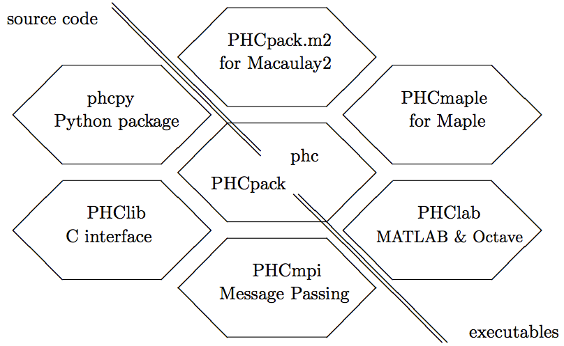
Fig. 1 Interfaces either require the source code or only the executable.

The interfaces PHCpack.m2, PHCmaple, PHClab, shown to the right of the antidiagonal require only the executable version phc. The other interfaces PHClib, PHCmpi, and phcpy are tied to the source code.

The phc.py (observe the dot between phc and py) is an optional package, available in the distribution of SageMath. Another, perhaps more natural interface to SageMath, is to extend the Python interpreter of SageMath with phcpy.

Runs in a Jupyter notebook work with a Python or SageMath kernel, using the interpreter with phcpy installed. For Julia, use PHCpack.jl, either as standalone or in a Jupyter notebook with a Julia kernel.

The Blackbox Solvers

Depending on whether the polynomial system has only isolated solutions, or whether also positive dimensional solution sets, select one of those two blackbox options:

1. phc -b to approximate all isolated solutions; or

2. phc -B for a numerical irreducible decomposition.

To use phc -b on the system we saved earlier in the file multilin, we invoke the blackbox solver typing at the command prompt

phc -b multilin multilin.phc

The output of the solver will be sent to the file multilin.phc. In case the input file did not yet contain any solutions, the solution list will be appended to the input file.

The output can also appear directly on screen, if the name of the output file is omitted at the command line.

We now explain the format of the solutions, for example, the last solution in the list occurs in the following format:

solution 44 :    start residual :  1.887E-14   #iterations : 1   success
t :  1.00000000000000E+00   0.00000000000000E+00
m : 1
the solution for t :
 a :  5.50304308029581E+00  -6.13068078142107E-44
 b :  8.32523889626848E+00  -5.18918337570284E-45
 c :  1.01021324864917E+01  -1.29182202179944E-45
 d :  1.42724963260133E+01   1.38159270467025E-44
 f :  4.34451307203401E+01  -6.26380413553193E-43
== err :  3.829E-12 = rco :  3.749E-03 = res :  2.730E-14 = real regular ==

This is the actual output of the root refiner. As the residual at the end of the solution path and at the start of the root refinement is already 1.887E-14, one iteration of Newton’s method suffices to confirm the quality of the root.

The next line in the output indicates that we reached the end of the path, at t :  1.00000000000000E+00   0.00000000000000E+00 properly. The multiplicity of the root is one, as indicated by m : 1. Then we see the values for the five variables, as pairs of two floating-point numbers: the real and imaginary part of each value. The last line summarizes the numerical quality of the root. The value for err is the magnitude of the last correction term used in Newton’s method. The number for rco is an estimate for the inverse condition number of the root. Here this means that we are guaranteed to have all decimal places correct, except for the last three decimal places. The last number represents the residual, the magnitude of the vector evaluated at the root.

The blackbox solver has two other interesting options:

1. To change the default working precision from hardware double precision into double double or quad double precision, call phc respectively with the options -b2 or -b4.

2. To use multiple threads in the solver, call phc with the option -t immediately followed by the number of threads. For example, to run the blackbox solver on 4 threads, type phc -b -t4.

Those two options may be combined. For example phc -b2 -t8 runs the blackbox solver on 8 threads in double double precision. If the computer has 8-core processors available, then phc -b2 -t8 may compensate for the overhead of double double arithmetic and be just as fast as the phc -b in double precision.

For the system adjmin4 above, representing the equations defining the adjacent 2-by-2 minors of a general 2-by-4 matrix, running phc -b does not make sense, as there are no isolated solutions. Instead, we can compute a numerical irreducible decompsition with the option -B, typing at the command prompt

phc -B adjmin4 adjmin4.phc

The user is then prompted to enter the top dimension of the solution set, which by default equals the number of variables minus one.

For this system, the output file will show that the solution set is a 5-dimensional solution set of degree 8, which factors into three irreducible components, of degrees 2, 2, and 4.

Double double, quad double, and multithreading is also supported in the numerical irreducible decomposition. To run in quad double precision on 16 threads, type phc -B4 -t16 at the command prompt.

Running the Program in Full Mode

If we just type in phc without any option, we run the program in full mode and will pass through all the main menus. A nice application is the verification of the counterexample of Bertrand Haas. We type in haas when the program asks us for the name of the input file. As the output may be rather large, we better save the output file on /tmp. As we run through all the menus, for this system, a good choice is given by the default, so we can type in 0 to answer every question. At the very end, for the output format, it may be good to type in 1 instead of 0, so we can see the progress of the program as it adds solution after solution to the output file.

If we look at the output file for the system in multilin, then we see that the mixed volume equals the 4-homogeneous Bezout number. Since polyhedral methods (e.g. to compute the mixed volume) are computationally more expensive than the solvers based on product homotopies, we can solve the same problem faster. If we run the program on the system in multilin in full mode, we can construct a multi-homogeneous homotopy as follows. At the menu for Root Counts and Method to Construct Start Systems, we type in 1 to select a multi-homogeneous Bezout number. Since there are only 52 possible partitions of a set of four unknowns, it does not take that long for the program to try all 52 partitions and to retain that partition that yields the lowest Bezout number. Once we have this partition, we leave the root counting menu with 0, and construct a linear-product system typing 2 in the menu to construct m-homogeneous start systems. We can save the start system in the file multilin_start (only used for backup). Now we continue just as before.

Running Toolbox Mode

The blackbox mode makes a selection of algorithms and runs them with default settings of the tolerances and parameters. In toolbox mode, defaults can be alterned and the stages in the solver are separated.

For Isolated Solutions Only

Skipping the preconditioning stage (scaling and reduction), we can compute root counts and construct start systems via the option -r, thus calling the program as phc -r. One important submenu is the mixed-volume computation, invoked via phc -m.

Once we created an appropriate start system, we can call the path trackers via the option -p. Calling the program as phc -p is useful if we have to solve a slightly modified problem. For instance, suppose we change the coefficients of the system in multilin, then we can still use multilin_start to solve the system with modified coefficients, using the -p option. In this way we use a cheater’s homotopy, alternatively called coefficient-parameter polynomial continuation.

Computing Components of Solutions

Consider the system of adjacent minors, we previously saved as adjmin4. We first must construct a suitable embedding to get to a system with as many equations as unknowns. We call phc -c and type 5 as top dimension. The system the program produces is saved as adjmin4e5. The blackbox solver has no difficulty to solve this problem and appends the witness points to the file adjmin4e5. To compute the irreducible decomposition, we may use the monodromy breakup algorithm, selecting 2 from the menu that comes up when we run with the option -f.