All Lines Tangent to Four Spheres

Consider all tangent lines to four mutually touching spheres.

The original formulation as polynomial system came from Cassiano Durand, then at the CS department in Purdue. The positioning of the centers of the spheres, each with radius 0.5 at the vertices of a tetrahedron came from Thorsten Theobald, then at TU Muenich. The centers of the four spheres are

\[c_1 = (0, 0, 0), \quad c_2 = (1, 0, 0), \quad c_3 = (1/2, \sqrt{3}/2, 0), \quad c_4 = (1/2, \sqrt{3}/6, \sqrt{6}/3).\]

Let \(t = (x_0, x_1, x_2)\) be the tangent vector and \(m = (x_3, x_4, x_5)\) the moment vector.

The first equation is \(\|t\|=1\), the second \(m \cdot t = 0\), the other equations are \(\|m - c_i \times t \|^2 - r^2 = 0\) where the radius \(r = 1/2\).

from sympy import var, sqrt
from sympy.vector import CoordSys3D, Vector
import matplotlib.pyplot as plt
import numpy as np

from phcpy.solver import solve
from phcpy.solutions import coordinates

centers and radii

Choices of the centers and radii of four mutually tangent spheres are defined here.

ctr1 = (0, 0, 0)
ctr2 = (1, 0, 0)
ctr3 = (0.5, sqrt(3.0)/2, 0)
ctr4 = (0.5, sqrt(3.0)/6, sqrt(6.0)/3)
radius = 0.5
centers = [ctr1, ctr2, ctr3, ctr4]

The choices were made for the suitability of the plot. Other choices can be found in the paper by Frank Sottile and Thorsten Theobald: Line problems in nonlinear computational geometry. In Computational Geometry - Twenty Years Later, pages 411-432, edited by J.E. Goodman, J. Pach, and R. Pollack, AMS, 2008.

formulating the equations

We need some vector calculus, done with sympy.

N = CoordSys3D('N')
x0, x1, x2 = var('x0, x1, x2')
vt = Vector.zero + x0*N.i + x1*N.j + x2*N.k
normt = vt.dot(vt) - 1
normt

which produces the first equation

x0**2 + x1**2 + x2**2 - 1

The second equation is

x0*x3 + x1*x4 + x2*x5

is computed by the code

x3, x4, x5 = var('x3, x4, x5')
vm = Vector.zero + x3*N.i + x4*N.j + x5*N.k
momvt = vt.dot(vm)

The radii are [0.5, 0.5, 0.5, 0.5] defined by

radii = [radius for _ in range(4)]

The polynomial system is constructed by

eqs = [normt, momvt]
for (ctr, rad) in zip(centers, radii):
    vc = Vector.zero + ctr[0]*N.i + ctr[1]*N.j + ctr[2]*N.k
    left = vm - vc.cross(vt)
    equ = left.dot(left) - rad**2
    eqs.append(equ)

To apply the blackbox solver, we have to convert the polynomials to strings.

fourspheres = []
print('the polynomial system :')
for pol in eqs:
    print(pol)
    fourspheres.append(str(pol) + ';')

The output to the above code cell is

the polynomial system :
x0**2 + x1**2 + x2**2 - 1
x0*x3 + x1*x4 + x2*x5
x3**2 + x4**2 + x5**2 - 0.25
x3**2 + (-x1 + x5)**2 + (x2 + x4)**2 - 0.25
(-0.866025403784439*x2 + x3)**2 + (0.5*x2 + x4)**2 + (0.866025403784439*x0 - 0.5*x1 + x5)**2 - 0.25
(-0.816496580927726*x0 + 0.5*x2 + x4)**2 + (0.288675134594813*x0 - 0.5*x1 + x5)**2 + (0.816496580927726*x1 - 0.288675134594813*x2 + x3)**2 - 0.25

So, we have six polynomial equations in six unknowns.

solving the problem

Now we call the blackbox solver.

sols = solve(fourspheres)

for (idx, sol) in enumerate(sols):
    print('Solution', idx+1, ':')
    print(sol)

The solution list is shown below:

Solution 1 :
t :  1.00000000000000E+00   0.00000000000000E+00
m : 4
the solution for t :
 x0 :  1.82013100766029E-16   2.92227989168779E-16
 x1 : -8.16496580927726E-01  -2.50326444773076E-17
 x2 : -5.77350269189626E-01   3.54015053218724E-17
 x3 :  6.04879596033482E-17   3.06586029409515E-17
 x4 :  2.88675134594813E-01  -1.77007526609362E-17
 x5 : -4.08248290463863E-01  -1.25163222386536E-17,
== err :  4.981E-16 = rco :  1.657E-17 = res :  3.821E-16 =
Solution 2 :
t :  1.00000000000000E+00   0.00000000000000E+00
m : 4
the solution for t :
 x0 : -7.07106781186547E-01  -2.17839875856796E-16
 x1 : -4.08248290463863E-01   2.08243914343071E-16
 x2 :  5.77350269189626E-01  -1.19547586767375E-16
 x3 :  2.50000000000000E-01  -3.72860037233369E-31
 x4 : -4.33012701892219E-01   2.77333911991762E-31
 x5 : -1.99196604815539E-16   2.50510368981921E-16
== err :  1.118E-15 = rco :  2.133E-17 = res :  4.441E-16 =
Solution 3 :
t :  1.00000000000000E+00   0.00000000000000E+00
m : 4
the solution for t :
 x0 :  7.07106781186547E-01   1.37982017054626E-16
 x1 : -4.08248290463863E-01   3.39894708038934E-18
 x2 :  5.77350269189626E-01  -1.66589349202482E-16
 x3 :  2.50000000000000E-01  -4.09837892165604E-31
 x4 : -1.44337567297407E-01   1.66589349202482E-16
 x5 : -4.08248290463863E-01  -5.88982292472640E-17
== err :  1.023E-15 = rco :  4.667E-17 = res :  3.331E-16 =
Solution 4 :
t :  1.00000000000000E+00   0.00000000000000E+00
m : 4
the solution for t :
 x0 : -7.07106781186547E-01   8.51323534940577E-17
 x1 :  4.08248290463863E-01  -9.82010876877884E-18
 x2 : -5.77350269189626E-01  -1.11209278833498E-16
 x3 : -2.50000000000000E-01   6.61657084254124E-29
 x4 :  1.44337567297406E-01   1.11209278833581E-16
 x5 :  4.08248290463863E-01  -3.93184175971020E-17
== err :  2.006E-14 = rco :  1.477E-17 = res :  5.551E-16 =
Solution 5 :
t :  1.00000000000000E+00   0.00000000000000E+00
m : 4
the solution for t :
 x0 :  7.07106781186548E-01   2.00971395228568E-16
 x1 :  4.08248290463863E-01  -2.45578336010813E-16
 x2 : -5.77350269189626E-01   7.24885788968468E-17
 x3 : -2.50000000000000E-01  -2.77333911991762E-31
 x4 :  4.33012701892219E-01  -3.82104500966428E-31
 x5 : -7.32462262249068E-17  -2.71206918859082E-16
== err :  7.741E-16 = rco :  4.417E-17 = res :  3.886E-16 =
Solution 6 :
t :  1.00000000000000E+00   0.00000000000000E+00
m : 4
the solution for t :
 x0 : -3.22358540809185E-16   5.45289082605370E-16
 x1 :  8.16496580927726E-01  -1.64014136987415E-17
 x2 :  5.77350269189625E-01   2.31951016948522E-17
 x3 : -1.74561355056418E-16   2.00875473111053E-17
 x4 : -2.88675134594813E-01  -1.15975508474262E-17
 x5 :  4.08248290463863E-01  -8.20070684937081E-18
== err :  5.471E-16 = rco :  1.448E-17 = res :  3.682E-16 =

Observe the m : 4 which indicates the multiplicy four of each solution.

the tangent lines

The solutions contain the components of the tangent and the moment vectors from which the tangent lines can be computed.

def tangent_lines(solpts, verbose=True):
    """
    Given in solpts is the list of solution points,
    the tuples which respresent the tangent lines
    are returned in a list.
    Each tuple contains a point on the line
    and the tangent vector.
    """
    result = []
    for point in solpts:
        if verbose:
            print(point, end='')
        tan = Vector.zero + point[0]*N.i + point[1]*N.j + point[2]*N.k
        mom = Vector.zero + point[3]*N.i + point[4]*N.j + point[5]*N.k
        pnt = tan.cross(mom) # solves m = p x t
        pntcrd = (pnt.dot(N.i), pnt.dot(N.j), pnt.dot(N.k))
        tancrd = (tan.dot(N.i), tan.dot(N.j), tan.dot(N.k))
        if verbose:
            print(', appending :', pntcrd)
        result.append((pntcrd, tancrd))
    return result

The input to the tangent_lines function is computed below:

crd = [coordinates(sol) for sol in sols]
complexpoints = [values for (names, values) in crd]
points = []
for point in complexpoints:
    vals = []
    for values in point:
        vals.append(values.real)
    points.append(tuple(vals))

and then the tangents are computed as

tangents = tangent_lines(points)

plotting the lines

Let us first plot the four spheres…

%matplotlib widget
fig = plt.figure()
ax = fig.add_subplot(projection='3d')
u = np.linspace(0, 2 * np.pi, 100)
v = np.linspace(0, np.pi, 100)
R = float(radius)
x1 = float(ctr1[0]) + R * np.outer(np.cos(u), np.sin(v))
y1 = float(ctr1[1]) + R * np.outer(np.sin(u), np.sin(v))
z1 = float(ctr1[2]) + R * np.outer(np.ones(np.size(u)), np.cos(v))
x2 = float(ctr2[0]) + R * np.outer(np.cos(u), np.sin(v))
y2 = float(ctr2[1]) + R * np.outer(np.sin(u), np.sin(v))
z2 = float(ctr2[2]) + R * np.outer(np.ones(np.size(u)), np.cos(v))
x3 = float(ctr3[0]) + R * np.outer(np.cos(u), np.sin(v))
y3 = float(ctr3[1]) + R * np.outer(np.sin(u), np.sin(v))
z3 = float(ctr3[2]) + R * np.outer(np.ones(np.size(u)), np.cos(v))
x4 = float(ctr4[0]) + R * np.outer(np.cos(u), np.sin(v))
y4 = float(ctr4[1]) + R * np.outer(np.sin(u), np.sin(v))
z4 = float(ctr4[2]) + R * np.outer(np.ones(np.size(u)), np.cos(v))
# Plot the surfaces
sphere1 = ax.plot_surface(x1, y1, z1, alpha=0.8)
sphere2 = ax.plot_surface(x2, y2, z2, alpha=0.8)
sphere3 = ax.plot_surface(x3, y3, z3, alpha=0.8)
sphere3 = ax.plot_surface(x4, y4, z4, alpha=0.8)
# Set an equal aspect ratio
ax.set_aspect('equal')
plt.show()

The output of the code cell is in Fig. 12.

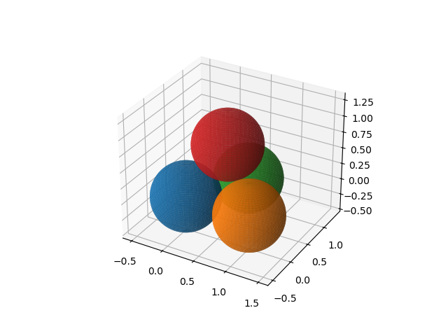
Fig. 12 Four touching spheres.

The second figure in Fig. 13 shows the tangent lines.

%matplotlib widget
ax = plt.figure().add_subplot(projection='3d')
# range of the tangent lines
theta = np.linspace(-2.5, 2.5, 10)
pnt1, tan1 = tangents[0]
x1 = float(pnt1[0]) + theta*tan1[0]
y1 = float(pnt1[1]) + theta*tan1[1]
z1 = float(pnt1[2]) + theta*tan1[2]
pnt2, tan2 = tangents[1]
x2 = float(pnt2[0]) + theta*tan2[0]
y2 = float(pnt2[1]) + theta*tan2[1]
z2 = float(pnt2[2]) + theta*tan2[2]
pnt3, tan3 = tangents[2]
x3 = float(pnt3[0]) + theta*tan3[0]
y3 = float(pnt3[1]) + theta*tan3[1]
z3 = float(pnt3[2]) + theta*tan3[2]
pnt4, tan4 = tangents[3]
x4 = float(pnt4[0]) + theta*tan4[0]
y4 = float(pnt4[1]) + theta*tan4[1]
z4 = float(pnt4[2]) + theta*tan4[2]
pnt5, tan5 = tangents[4]
x5 = float(pnt5[0]) + theta*tan5[0]
y5 = float(pnt5[1]) + theta*tan5[1]
z5 = float(pnt5[2]) + theta*tan5[2]
pnt6, tan6 = tangents[5]
x6 = float(pnt6[0]) + theta*tan6[0]
y6 = float(pnt6[1]) + theta*tan6[1]
z6 = float(pnt6[2]) + theta*tan6[2]
line1 = ax.plot(x1, y1, z1)
line2 = ax.plot(x2, y2, z2)
line3 = ax.plot(x3, y3, z3)
line4 = ax.plot(x4, y4, z4)
line5 = ax.plot(x5, y5, z5)
line6 = ax.plot(x6, y6, z6)
# Set an equal aspect ratio
ax.set_aspect('equal')
plt.show()

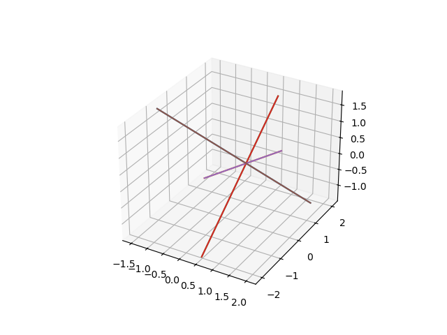
Fig. 13 The computed tangent lines.

And then we plot the spheres and the tangent lines:

%matplotlib widget
fig = plt.figure()
ax = fig.add_subplot(projection='3d')
u = np.linspace(0, 2 * np.pi, 100)
v = np.linspace(0, np.pi, 100)
R = float(radius)
x1 = float(ctr1[0]) + R * np.outer(np.cos(u), np.sin(v))
y1 = float(ctr1[1]) + R * np.outer(np.sin(u), np.sin(v))
z1 = float(ctr1[2]) + R * np.outer(np.ones(np.size(u)), np.cos(v))
x2 = float(ctr2[0]) + R * np.outer(np.cos(u), np.sin(v))
y2 = float(ctr2[1]) + R * np.outer(np.sin(u), np.sin(v))
z2 = float(ctr2[2]) + R * np.outer(np.ones(np.size(u)), np.cos(v))
x3 = float(ctr3[0]) + R * np.outer(np.cos(u), np.sin(v))
y3 = float(ctr3[1]) + R * np.outer(np.sin(u), np.sin(v))
z3 = float(ctr3[2]) + R * np.outer(np.ones(np.size(u)), np.cos(v))
x4 = float(ctr4[0]) + R * np.outer(np.cos(u), np.sin(v))
y4 = float(ctr4[1]) + R * np.outer(np.sin(u), np.sin(v))
z4 = float(ctr4[2]) + R * np.outer(np.ones(np.size(u)), np.cos(v))
# Plot the surfaces
sphere1 = ax.plot_surface(x1, y1, z1, alpha=0.8)
sphere2 = ax.plot_surface(x2, y2, z2, alpha=0.8)
sphere3 = ax.plot_surface(x3, y3, z3, alpha=0.8)
sphere4 = ax.plot_surface(x4, y4, z4, alpha=0.8)
# range of the tangent lines
theta = np.linspace(-2.5, 2.5, 10)
pnt1, tan1 = tangents[0]
x1 = float(pnt1[0]) + theta*tan1[0]
y1 = float(pnt1[1]) + theta*tan1[1]
z1 = float(pnt1[2]) + theta*tan1[2
pnt2, tan2 = tangents[1]
x2 = float(pnt2[0]) + theta*tan2[0]
y2 = float(pnt2[1]) + theta*tan2[1]
z2 = float(pnt2[2]) + theta*tan2[2]
pnt3, tan3 = tangents[2]
x3 = float(pnt3[0]) + theta*tan3[0]
y3 = float(pnt3[1]) + theta*tan3[1]
z3 = float(pnt3[2]) + theta*tan3[2]
pnt4, tan4 = tangents[3]
x4 = float(pnt4[0]) + theta*tan4[0]
y4 = float(pnt4[1]) + theta*tan4[1]
z4 = float(pnt4[2]) + theta*tan4[2]
pnt5, tan5 = tangents[4]
x5 = float(pnt5[0]) + theta*tan5[0]
y5 = float(pnt5[1]) + theta*tan5[1]
z5 = float(pnt5[2]) + theta*tan5[2]
pnt6, tan6 = tangents[5]
x6 = float(pnt6[0]) + theta*tan6[0]
y6 = float(pnt6[1]) + theta*tan6[1]
z6 = float(pnt6[2]) + theta*tan6[2]
line1 = ax.plot(x1, y1, z1)
line2 = ax.plot(x2, y2, z2)
line3 = ax.plot(x3, y3, z3)
line4 = ax.plot(x4, y4, z4)
line5 = ax.plot(x5, y5, z5)
line6 = ax.plot(x6, y6, z6)
# Set an equal aspect ratio
ax.axes.set_xlim3d(-1.5, 1.5)
ax.axes.set_ylim3d(-1.5, 1.5)
ax.axes.set_zlim3d(-1.5, 1.5)
ax.set_aspect('equal')
ax.view_init(elev=30, azim=30, roll=0)
plt.show()

which produces Fig. 14.

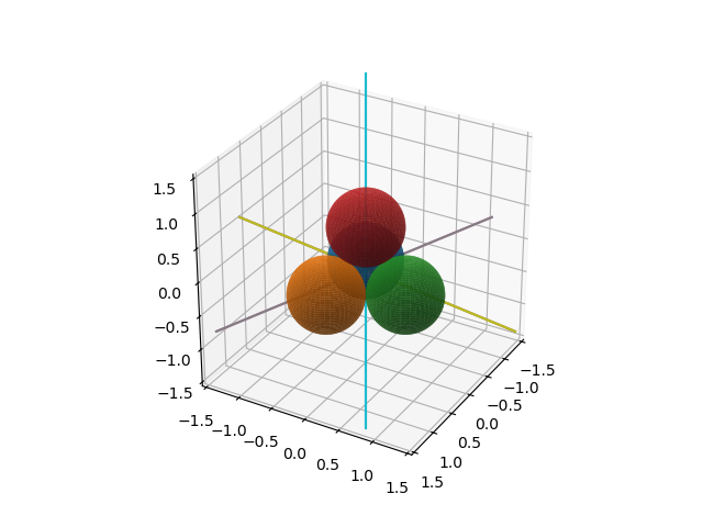
Fig. 14 All lines tangent to four spheres.