A Counter Example to Koushnirenko’s Conjecture
This chapter illustrates the counter example of Bertrand Haas, against the Koushnirenko conjecture, executed on one core and on many cores. For the mathematical background, consult:
Bertrand Haas: A simple counterexample to Kouchnirenko’s conjecture., Beitraege zur Algebra und Geometrie/Contributions to Algebra and Geometry, volume 43, number 1, pages 1 to 8, 2002.
Bertrand constructed a polynomial system with three monomials in every equation and with five positive real roots. Kouchnirenko’s conjecture predicted there could only four positive real roots for such a system.
To get the proper wall clock time, we have to be mindful
that the Python code calls the compiled functions in the PHCpack library.
Therefore, the Python timers will not give accurate timings.
Instead, we have to rely on the actual date and time,
from the package datetime in Python.
from datetime import datetime
For the plot, the implicit plotting of sympy will be used.
from sympy import plot_implicit, symbols, Eq
From phcpy we import the following functions:
from phcpy.dimension import get_core_count
from phcpy.solver import solve
from phcpy.solutions import filter_real
solving the system on many cores
The example of Bertrand Haas is defined as
H = [ 'x**108 + 1.1*y**54 - 1.1*y;',
      'y**108 + 1.1*x**54 - 1.1*x;' ]
According to the theorem of Bézout, we may expect a number of complex solutions equals to the product of the degrees of the polynomials. The square of 108 equals 11664. As the solver computes all complex solutions, executing the following code block takes some time …
print('Solving on one core ...')
wstart = datetime.now()
sols = solve(H)
wstop = datetime.now()
print('  Number of solutions :', len(sols))
print('start time :', wstart)
print(' stop time :', wstop)
print('   elapsed :', wstop - wstart)
The output of the above code cell is
Solving on one core ...
  Number of solutions : 11664
start time : 2024-01-28 11:57:53.061707
 stop time : 2024-01-28 11:57:59.223344
   elapsed : 0:00:06.161637
We can significantly speed up this computation if the computer has many cores.
nbcores = get_core_count()
print('Solving on', nbcores, 'cores ...')
wstart = datetime.now()
sols = solve(H, tasks=nbcores)
wstop = datetime.now()
print('  Number of solutions :', len(sols))
print('start time :', wstart)
print(' stop time :', wstop)
print('   elapsed :', wstop - wstart)
The output of the above code cell is
Solving on 32 cores ...
  Number of solutions : 11664
start time : 2024-01-28 11:58:07.241324
 stop time : 2024-01-28 11:58:08.747874
   elapsed : 0:00:01.506550
Compared the elapsed : above with the previous one.
extracting the real roots
Rather than eyeballing all 11,664 complex solutions ourselves, we ask to filter the real solutions.
realsols = filter_real(sols, tol=1.0e-8, oper='select')
The code cell below prints the solutions in realsols:
for (idx, sol) in enumerate(realsols):
    print('Solution', idx+1, ':')
    print(sol)
The output is
Solution 1 :
t :  0.00000000000000E+00   0.00000000000000E+00
m : 1
the solution for t :
 x :  0.00000000000000E+00   0.00000000000000E+00
 y :  0.00000000000000E+00   0.00000000000000E+00
== err :  0.000E+00 = rco :  1.000E+00 = res :  0.000E+00 =
Solution 2 :
t :  1.00000000000000E+00   0.00000000000000E+00
m : 1
the solution for t :
 x :  9.91489402484465E-01  -2.94004118110142E-49
 y :  9.91489402484465E-01   2.96676882820234E-49
== err :  7.704E-17 = rco :  8.274E-02 = res :  5.773E-15 =
Solution 3 :
t :  1.00000000000000E+00   0.00000000000000E+00
m : 1
the solution for t :
 x :  9.99997917489999E-01   9.52445049970774E-46
 y :  9.19904793199125E-01  -1.72639970804817E-42
== err :  2.708E-16 = rco :  1.601E-03 = res :  8.677E-15 =
Solution 4 :
t :  1.00000000000000E+00   0.00000000000000E+00
m : 1
the solution for t :
 x :  9.99986016402972E-01   1.19248391761152E-37
 y :  9.36266084294562E-01  -2.97164971887874E-34
== err :  2.240E-15 = rco :  2.070E-03 = res :  3.610E-15 =
Solution 5 :
t :  1.00000000000000E+00   0.00000000000000E+00
m : 1
the solution for t :
 x :  9.19904793199125E-01  -2.01786978862774E-41
 y :  9.99997917489999E-01   1.02032044433651E-44
== err :  4.384E-16 = rco :  1.601E-03 = res :  8.564E-15 =
Solution 6 :
t :  1.00000000000000E+00   0.00000000000000E+00
m : 1
the solution for t :
 x :  9.36266084294562E-01  -4.40471624223194E-48
 y :  9.99986016402972E-01   3.13214614463929E-51
== err :  9.256E-17 = rco :  2.070E-03 = res :  3.730E-15 =
We observe (0, 0) and five additional real positive roots. According to the Koushnirenko conjecture, we would expect no more than four real positive roots.
plotting the curves
In converting the strings in the polynomial system H
we have to remove the trailing semicolon
x, y = symbols('x y')
p0 = eval(H[0][:-1])
p1 = eval(H[1][:-1])
Without knowing the precise location of the intersection points, the curves are hard to plot. The code below produces the plot Fig. 1.
plot0 = plot_implicit(Eq(p0, 0), (x, 0.93, 1.01), (y, 0.93, 1.01),
                      line_color='black', depth=1,
    markers=[{'args': [[0.99148, 0.93626, 0.99998],
                       [0.99148, 0.99998, 0.93626], 'bo']}],
                      axis_center=(0.93, 0.93), show=False)

plot1 = plot_implicit(Eq(p1, 0), (x, 0.93, 1.01), (y, 0.93, 1.01),
                      line_color='red', depth=1,
                      axis_center=(0.93, 0.93), show=False)

plot0.append(plot1[0])
plot0.show()
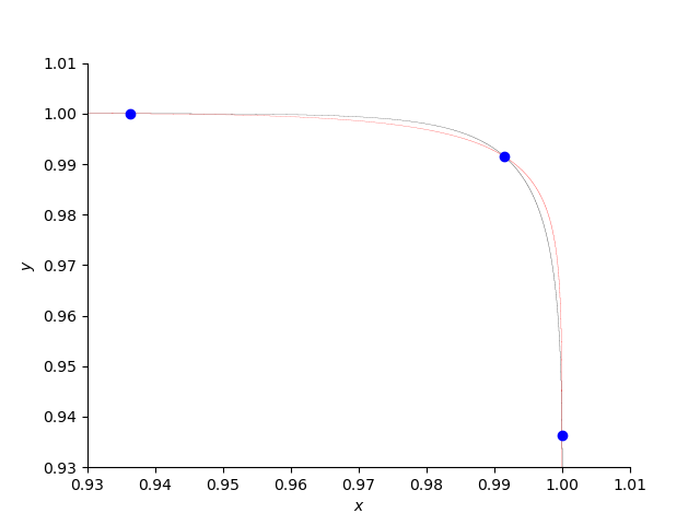
Fig. 1 Three positive roots of the counterexample.
Let us zoom in to another root … Fig. 2 is made executing the code below:
plot3 = plot_implicit(Eq(p0, 0), (x, 0.9, 1.0025), (y, 0.99, 1.0025),
                      line_color='black', depth=1,
    markers=[{'args': [[0.99148, 0.93626, 0.91990],
                       [0.99148, 0.99998, 0.99999], 'bo']}],
                      axis_center=(0.9, 0.99), show=False)

plot4 = plot_implicit(Eq(p1, 0), (x, 0.9, 1.0025), (y, 0.99, 1.0025),
                      line_color='red', depth=1,
                      axis_center=(0.9, 0.99), show=False)

plot3.append(plot4[0])
plot3.show()
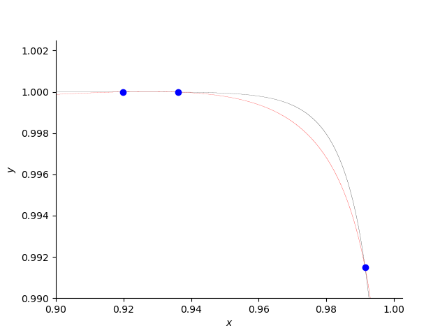
Fig. 2 Other positive roots of the counterexample.
The third plot (in Fig. 3) is produced by the following code:
plot5 = plot_implicit(Eq(p0, 0), (x, 0.9, 1.0005), (y, 0.999, 1.0005),
                      line_color='black', depth=1,
    markers=[{'args': [[0.93626, 0.91990],
                       [0.99998, 0.99999], 'bo']}],
                      axis_center=(0.9, 0.999), show=False)

plot6 = plot_implicit(Eq(p1, 0), (x, 0.9, 1.0005), (y, 0.999, 1.0005),
                      line_color='red', depth=1,
                      axis_center=(0.9, 0.999), show=False)

plot5.append(plot6[0])
plot5.show()
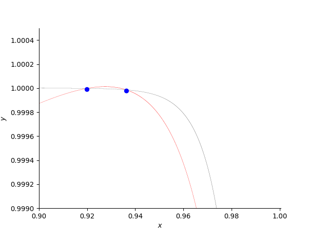
Fig. 3 Two close positive roots of the counterexample.