MthT 430 Notes Chapter 4a Graphs

Real Numbers and Points on a Line

The real numbers in R are identified with points on a horizontal line. For the time being, we will identify a real number x with a decimal expansion .

•

Every decimal expansion represents a real number x:

x = ±N.d1d2…, dk ∈ {0,1, ... ,9}.

This is the statement that every infinite series of the form

d1 10−1 + d2 10−2 + …,     dk ∈ {0,1, ... ,9},

converges.

Just as well we could identify a real number x with a binary expansion .

•

Every binary expansion represents a real number x:

x = ±N.binb1b2…, bk ∈ {0,1}.

This is the statement that every infinite series of the form

b1 2−1 + b2 2−2 + …,     bk ∈ {0,1},

converges.

A demonstration of a correspondence between the binary expansion and a point on a horizontal line was given in class. See also

chap4b.htm

Intervals

•

(a,b) ≡ {x | a < x < b} is the open interval from a to b. Usually it is assumed that a is less than b. If b < a, then (a,b) = ∅, the empty interval.

•

[a,b] ≡ {x | a ≤ x ≤ b} is the closed interval from a to b. Usually it is assumed that a is less than or equal b. If b < a, then [a,b] = ∅, the empty interval.

The "points" − ∞ and ∞ are introduced so that we have

•

(a,∞) ≡ {x | a < x } is the open interval from a to ∞.

•

(−∞, b] ≡ {x | x ≤ b } is the closed interval from −∞ to b.

•

(−∞, ∞) ≡ …

In graphing an interval, whether an endpoint is included or not is usually indicated by explicitly drawing the point or placing a (, ), [, ], •, or ° at the indicated coordinate.

See the examples in Spivak, pp. 50 ff.

Note the equations (formulas) for lines.

If the function is defined on the closed interval between two points points x, x+ ∆x, let

∆f(x) = f(x + ∆x) − f(x).

Qualitative properties of graphs to be observed on intervals are

•

Continuity (to be defined precisely in Chapter 5) - ∆f(x) is small if ∆x is small. Note particular points where the function is not defined or is not continuous

•

Monotonicity - increasing or decreasing on particular intervals - ∆f(x) is of constant sign for all x, x+ ∆x in the interval with ∆x > 0

•

Concavity on particular intervals - for equal ∆x, ∆f(x) is increasing/decreasing as x increases in the interval.

Examples

•

Figure 20:

f(x) = sin ⎛ ⎝ 1 x ⎞ ⎠ .

With our convention, domain(f) = {x ≠ 0}. The intervals of increase and decrease are evident, concavity is not quite so clear.

•

The function sinxoverx:

sinxoverx (x) = ⎧ ⎪ ⎨ ⎪ ⎩ sin(x) x , x ≠ 0 undefined, x = 0.

•

The function Siprime:

Siprime(x) = ⎧ ⎪ ⎨ ⎪ ⎩ sin(x) x , x ≠ 0 1, x = 0.

The function Siprime(x) is an extension of the function sinxoverx, and is continuous at x = 0. At x = 0, for ∆x small about ≠ 0,

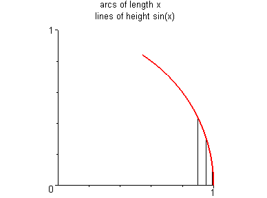
∆Siprime = Siprime(∆x) − Siprime(0) = sin(∆x) ∆x − 1 = |small line| |small arc| − 1 = small - draw a picture.

Here is the picture for the above calculation:

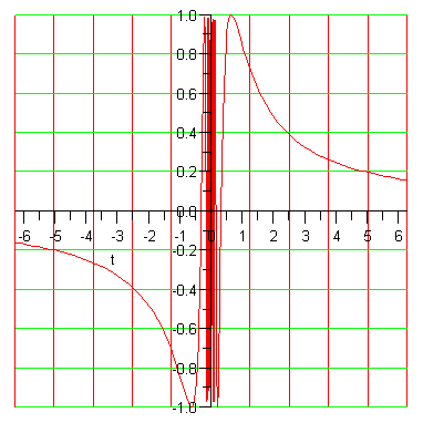
Here is the plot of sin([1/x]) on [− 2 π, 2 π]

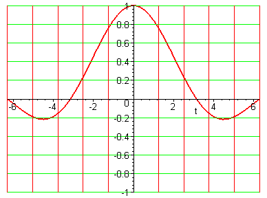
Here is the plot of Siprime(t) on [− 2 π, 2 π]

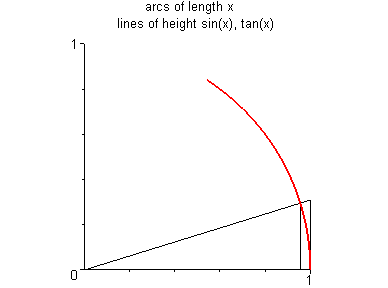
Here is another picture which shows that

lim x → 0  sin(x) x =1.

Note that, for x > 0, sin(x) < x < tan(x).

---

File translated from T_EX by T_TH, version 4.04.
On 22 Aug 2014, 13:51.