Pattern, Sign and Space

by Louis H. Kauffman

We have been investigating the "Pattern" for some years now, ever since Lynnclaire Dennis showed us her images, ideas and intuitions. There is something uniquely compelling about knots

in any case and certainly so for the first and simplest knot, the trefoil knot. The trefoil knot alone is not the pattern, but a form of the trefoil knot leads into the pattern, which is a weaving

of the trefoil knot in a dynamic and polyhedral context. Even this very specific three-dimensional articulation is not THE pattern, for what we are actually investigating is the way simple and

fundamental forms (particularly gemoetrical forms) act as pivots for ideas and understandings.

In the Sequoia Seminars we explicitly used Lynnclaire's Pattern as such a pivot, to bring together discussions as diverse as the structure of the symbolism of the Knights Templar, the use of

exceptional Lie algebras in the articulation of spacetime, the tensegrity structure of the living cell, the topology of knot energies, the role of the vector equilibrium in Buckminster Fuller

geometry and in the dynamics of polyhedra, the abstract foundations of quantum theory, foundations of discrete physics, the structure of deep dialogue.

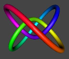
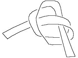
What you see in the figure above is a relatively stable self-repelling energy minimal form of the trefoil knot that evolved after starting it in the position of the (3,2) torus knot. This form above we have come to call the "Pattern" knot.

Above you see the relatively flat starting position called (3,2) winding three times around the axis parallel to your line of sight for two turns around an imaginary torus.

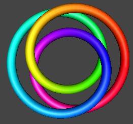
The reverse version with the same topology is the (2,3) shown below.

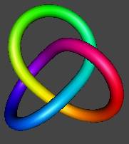
And the self-repelled form of the (2,3) is the most well-known form of the trefoil knot.

The Patttern knot is remarkable in that it is a nearly stable higher energy form of the trefoil knot, and it was in this form that Lynnclaire Dennis saw it in the context of polyhedral spheres.

There is a curious fascination with this domain that on the mathematical side is surely related to the fact that there are deep underlying relationships between the differential geometry and polydehral geometry of knots and their topological characteristics.

Beyond this, we found ourselves using this pictorial geometry as a jumping off point for many excursions into other areas of science.

We call this sort of excursion "investigating the Pattern" as though we knew what we were doing! And we do know, in the sense that we are allowing a free-wheeling association of patterns, with the intent to be critical in those ways that are appropriate to the domains encountered.

This quick tour through knots and knot energies gives one view of how we ended up investigating the pattern. There is another dimension of this invesitigation that lives in an unorthodox mixture of topology, combinatorics and mythological or methphorical thinking. Here the mathematics and geometry becomes a springboard for the discussion of ideas and connections.

Bateson: "The pattern that connects is a pattern of patterns."

I. From The Five Elements to the Petersen Graph and the Dodecahedron

I would like to illustrate some ways in which very simple patterns exfoliate in many directions with one example that is close to the usual three dimensional Mereon, but arises in a more abstract

way. Lets begin with the well-known Chinese Theory of the Five Elements: Wood, Fire, Earth, Metal, Water.

These elements are Qualities and yet are understood through their particulars as well as the generalities that lie behind them. Thus and for example Wood is associated with Spring, Fire with Summer, Earth with Change, Metal with Autumn, Water with Winter. In this form we see the generative cycle

where water nourishes growth producing wood; wood burns producing fire; the ashes of fire become earth; earth sources metal; metal can liquifiy and so return to the form of water. The cycle is not literal and it contains a meta-level within it (where we see molten metal and water as one through their common property of liquidity). In the cycle of seasons and change, Change herself is an element of the cycle along with the seasons. At a numerological level

FIVE is the first place where meta-level occurs and is included into the language of that level itself.

Along with the generative cycle, there is the cycle of destruction:

Here Wood can enter or penetrate the Earth; Earth can absorb Water, Water can put out Fire: Fire can melt Metal; Metal can splinter Wood.

The two cycles interpentrate and form the whole of the process of creation and destruction in the world so described.

Does this remind you of the Pattern?

Of course.

There are the two cycles.

One is an "inner sphere".

The other is an "outer shere".

By asking that the outer sphere be spherical

(that is, not self-crossing)

The inner cycle becomes a self-crossing star,

A relative of a knot

And likely to be drawn in knotted form.

In this sense the "knot" arises in the

Interaction of the two

Cycles (spheres).

Pattern herself, being three dimensional and quite capacious

can accomodate easily the mythology of the Cycles of the Five Elements. But this is not quite my point!

A few days ago (December 12, 2002) I looked at that

diagram of the two cycles and recognized it as an old friend from the graph theory!

Above you will see a drawing of the cycle diagram in the form of a "graph". In a graph there are "nodes" (the small dark disks) and "edges" the line segments that connect pairs of dark disks. This graph has ten nodes and 15 edges. Note that some nodes are connected to each other by edges and some are not connected. In this graphical depiction the designations Wood, Fire, Earth, Metal, Water each refer to two nodes, one on the outer creative cycle and one on the inner destructive cycle. In our previous diagram we had associate points on the inner cycle with points on the outer cycle by enclosing them in circles. Now they are joined by edges, and we must see these edges as playing a differenct role than the edges of the two cycles. Among graph theorists, this graph is called the Petersen graph after a theorist named Petersen who discovered it and its remarkable mathematical properties at the end of the nineteenth century.

I was startled to realize that Petersen's Graph in its essential structure had been known to the ancient Chinese. They surely did not know about its mathematical secrets (that I shall soon reveal), but now we must ask if these mathematical secrets are related to the deep generalities of the Theory of the Five Elements.

This is a microcosm of the sort of investigation that we are involved in with the Pattern. It is also part of that investigation.

First of all, the Petersen graph does not come with labels. It is just the node and vertex structure itself.

Second, as an abstract structure of nodes and edges, the Petersen is completeley symmetric. It looks exactly the same when viewed from any node. You might think that the nodes of the outer five cycle have a priviledged position with respect to the nodes of the inner five cycle, but this is not so. View the figure below.

Here we see that one can exchange the outer and inner cycles, maintaining the same graphical relationships (except for a change from clockwise to anticlockwise in the plane for the outer cycle).

In fact, the Petersen graph is a close relative of the graphical structure of the Dodecahedron (depicted above). The dodecahedron is one of the five Platonic solids, a regular polyhedron with pentangonal faces, and three pentagons surrounding each node. On the surface of this polyhedron there are 12 pentagonal faces, 20 nodes and 30 edges. Thinking of the dodecahedron as describing the surface of a sphere, we can ask what graphical structure will result from identifying antipodal points on the surface of that sphere. The answer is the Petersen graph! I will leave this as an exercise for the reader, but note that the Petersen graph has 10 nodes and 15 edges, just half of the corresponding number for the dodecahedron. One way to visualize this identification of antipodal points is to realize that the resulting graphical structure is obtained from the upper hemisphere by identifying antipodal points along the equator. The result of this identification is shown in the figure below.

In this figure I have indicated the upper hemisphere of the dodecahedron, and the edges that must be identified to one another along the equator, in order to complete the antipodal identification from the dodecahedron. The result of completing these identifications is shown below, and it is apparent that we have arrived at the Petersen graph!

In this way we see the Petersen graph as a descendant of a classical geometric construction in three dimensional space, but more should be said about this operation of antipodal identification, for it is central to the notion a projective geometry, a more modern notion coming from the eighteenth century!

So now we digress about projective geometry: In developing the practice of perspective drawing artists realized the utility of indicating points that are effectively at infinity for a given observer.

Thus one draws a horizon line where parallel lines meet in the drawing. In actual space (also idealized) the parallel lines never meet.

Adding ideal points where parallel lines meet changes the topology of space to that of a "projective space". We imagine that any two parallel lines in the plane meet at a unique point at infinity. This means that the infinite extension of a line in the forward direction meets the infinite extension of that line in the backward direction.

We can make a finite model of the projective space by thinking about the lines going through the origin in three dimensional sapce. Each such line partakes of a unique point at infinity and this point can be thought of as follows. First restrict all the lines to a ball about the origin of radius one. Then identify antipodal points on the boundary of this ball. The result for any given line through the origin is that it intesects the surface boundary of the ball in two points and these are identified with one another. The result is that each line through the origin is replaced by a circle, just as in the original projective space where one goes around the circle by heading out to infinity in the forward direction and returning from infinity from the backward direction.

This bundling up of the lines in the projective space makes it contain a Mobius band for each pair of parallel lines!

Now a Mobius band is a topological denizen of three dimensional space as illustrated above. It is obtained by taking a strip of paper and indentifying the ends after making a one-half twist. The Mobius is of interest because it has only one edge and only one side. Furthermore, if you cut the Mobius band down the middle, then the most mysterious thing happens. You had best try it.

But what does this have to do with parallel lines in projective space?

Well, it is like this: If you have two parallel lines then they meet at infinity. If you have two non-parallel lines then they cross over one another in finite space and so have to have a cross over identification from infinity as well.

All this is probably most clear if we resort to the model of the projective plane that is obtained from our three dimensional description above by taking a disk and identifying antipodal points along the boundary of the disk. A finite model would appear as below where we identify the intervals a,b,c,d,e with the arrows as shown.

Now look inside this model and you will "see" a Mobius strip M!

The region between the two dark lines labled L and R and bounded by the two copies of b is a Mobius strip. You can see this by just noting that the two copies of b have to be identified with each other and that the performing of this identification requires the twisting of this strip by one half twist, producing the Mobius band.

Lets summarize. Projective drawing leads to projective geometry, a realm where the ideal points at infinity are part of the space itself. Projective three space is a topologically equivalent to a ball with antipodal identifications on the boundary. The projective plane is topologically equivalent to a disk with antipodal identifications on its boundary.

The projective plane can also be described as the result of making antipodal identifications on the surface of a two dimensional sphere. The result of such idenitifications is the same as taking the upper hemisphere of that two sphere, and then making antpodal identifications one the boundary. This was our description of the projective plane.

The projective plane contains a Mobius strip, as does projective three space. But also, the Petersen graph is obtained from the graph of the dodecahedron by reagrding the graph of the dodecahedron as in the boundary of a three ball and making antipodal identifications in the boundary. In the light of the above discussion, this shows that if we take the dodecahedral graph as embedded in the surface of the two sphere, then the Petersen graph is embedded in the two dimensional projective space obtained by making antipodal identifications on the surface of that two sphere.

Is there a Mobius strip somwhere in the Petersen graph?!

The answer is yes, if you view the Petersen in the right way!

You can see how this is embedded in the projective plane as follows.

This rather Mondrian version of the Petersen graph is seen the in the projective plane by identifying antipodal points in the circle the figure. With the points labeled c and c, b and b, a and a indentified to one another we get an embedding of the Petersen graph in the projective plane. What happened to the interacting five cycles of the theory of the Chinese elements?

In the above figure you can see how the two five cycles in the original Petersen graph map to the five cycles in the embedding of the Petersen in the projective plane. Note again that the a's b's and c's are identified in pairs.

Another way to think about this view of the Petersen graph in terms of projective space is to go back to the dodecahedron, but label the five cycles on the dodec itself. Then there will be two repeats for each five cycle, since every point and edge of the Petersen graph is doubled when we use the dodecahedron.

Now we can ask again, what is the significance for the original cycle of the five elements in this representation? If we identify the cycle 12345 with the original cycle of creation, then we see that in the dodecahedron there are two complete copies of this cycle, one at the top of the dodecahedron and one at the bottom. The cycle of destruction is then 1'2'3'4'5' and this cycle appears in the dodecahedron twice also, but doubled, like a snake eating its tail in the form 1'2'3'4'5'1'2'3'4'5' around the equator. Furthermore, we see that the permutation of 1'2'3'4'5' that is associated to travel around the cycle 12345 is now displayed by skipping one number each time in the sequence 1'2'3'4'5'1'2'3'4'5' and writing the result in backwards order! Thus we start by skipping to produce 1' 3' 5' 2' 4'

and then reverse the order to get 4' 2' 5' 3' 1'. This is order of the encircled numbers going round in accord with the creation cycle 12345 as shown in the figure above. The cycle of destruction has taken an entirely different character in the dodecahedral graph and in this way our unfolding of the five elements into the dodecahedron adds to an understanding of its inherent structure.

The metaphor of the two spheres appears again with the two copies of the creation cycle taking the part of the two shpheres, and the single "self-knotted" equator forming the cycles of destruction that intermediate creation.

II. Coloring and the Petersen Graph

The Petersen graph became famous as an example of a minimal uncolorable non-planar graph. The coloring we are interested in is coloring of the edges of the graph with three colors (say r=red, b=blue, p = purple) so that three distinct colors appear at each node.

A cubic graph (three edges per vertex) is said to be properly colored if there is a coloring of its edges with these three colors such that every node sees three distinct colors. Note that in a proper coloring the colors will appear in a drawing of a node in one of the two ways depicted in the figure above. For example, the following graph is planar and colorable.

Here is a more complex example of a colorable graph.

Not all graphs are colorable. The simplest non-colorable graph possible is the dumbell shown below.

There is no way to color the dumbell graph because each node only allows two colors, and a proper coloring demands three colors at a node. Less than three is not good enough for a proper coloring.

In general, among graphs that might be colorable we must throw away graphs with "bridges" where a bridge is an edge that will disconnect the graph when it is deleted. The middle edge in the dumbell is a bridge and the dumbell becomes two disjoint circles when it is deleted.

One can show that any graph that has a bridge is neccessarily uncolorable whether it is planar or not. However the most famous theorem about cubic graphs is the

Cubic Graph Coloring Theorem. Every cubic connected bridgeless planar graph can be properly edge colored with three colors.

This theorem is logically equivalent to the famous Four Color Theorem for plane maps. I shall not explain that equivalence here.

The beauty of considering proper colorings of cubic maps is that one can see how to construct bridgeless connected uncolorables that are not planar, and so begin to see the relationship of planarity with this deep theorem. This is where the Petersen graph comes in.

In order to see how the Petersen enters this scene, I will introduce a little theory about coloring cubic graphs. Let a double arrow indicator between two graphical edges mean that these two edges are neccessarily colored differently. This means that we are selecting those colorings where the colors are different on the two arcs.

For example, we can write

The graph is colorable but in all colorings the indicated edges necessarily receive the same color (exercise!). Consequently, the presence of the double-arrow on this graph means that we are reduced to an empty set of colorings that satisfy this description. On the other hand, for the graph shown below there are colorings that satisfy the condtion and one such coloring is indicated on the graph.

We can now state the following

The Diagram Color Theorem. Let G be a connected cubic graph and let e be an edge in G. Then the set of colorings of G is in one-to-one correspondence with the set of colorings of G' and G'' where G' is the graph obtained from G by excising e and reconnecting with two parallel arcs, while G' is the graph obtained from G by excising e and reconnecting with two crossed arcs. In the graphs G' and G'' we only consider those colorings where the two arcs of reconnection receive different colors. Thus G' and G'' are graphs with an indicator attached showing which arcs must be colored differenctly. This statement is illustrated in the diagrammatic equation shown below.

In the diagrammatic statement, we have let C(G) denote the set of colorings of G and we have let the plus sign (+) denote disjoint union. Thus we can write C(G)= C(G') + C(G'').

Proof. The proof of this theorem follows at once from the fact that for any coloring of G, the two colors coming into one end of the edge e must be the same as the two colors adjacent to the other end of the edge e. In the diagrammatic formulation, the two colors at the top of the double y are either parallel or permuted from the two colors at the bottom of the double y. See the illustration below.

In the case where the colors are parallel, the coloring is induced by a coloring of G'. When the colors are permuted the coloring is induced by a coloring of G'', as shown below.

It is clear that this association produces the one-to-one correspondence asserted by the Theorem. QED

We can use this Theorem to investigate the structure of uncolorable graphs. Suppose that G is uncolorable and that any graph H with fewer nodes than G is colorable. I will call G a "minimal uncolorable" graph. We want to understand the structure of minimal uncolorable graphs. To this end here is a useful way to indicate any cubic graph.

In this diagram B is a "black box" containing all of G except the edges and nodes external to it. There are two nodes external to B and five edges. The diagram shows only how these edges terminate at the two nodes shown. The edges enter the black box at the corners of the box, but the bounding edges of the box are not necessarily edges of the graph G. The crossover between edges that is shown in G is useful for our purposes and there is no loss in generality since a cancelling crossover can be placed inside the box B if it is needed. Any cubic graph can be placed in the plane with the addition of a sufficient number of such crossovers. Of course a plane graph G can be represented without crossovers. We shall refer to the above diagram as a "template" for the graph G.

Here is a particularly simple template.

This template encapsulates a graph that is equivalent to the dumbell.

As we have seen before, the Petersen graph in its Mobius incarnation has the form of a template.

Now suppose that we are given G in the form of a template and that we apply the Diagram Theorem. to G.

Thus we conclude that

This final equation shows that the proper colorings of G are in one-to-one correspondence with the proper colorings of the two basic closures of the box B with the stipulation that the colors on the exposed edges must be unequal. We can write this as the equation

C(G(B)) = C(D*(B)) + C(N*(B)) where D*(B) and N*(B) denote the closures of B (with coloring stipulations) as shown in the above figure and G(B) denotes the template associated with the box B. We let D(B) and N(B) denote the graphs obtained from the denominator (D) and numerator (N) closures of the box B. Colorins of D(B) and N(B) can be performed without the restrictions imposed by the double arrows in

D*(B) and N*(B).

Now suppose that G(B) is uncolorable and minimal. Then N(B) and G(B) must both be colorable, but N*(B) and G*(B) are necessarily uncolorable (with stipulation) since G(B) is uncolorable. Therefore, both N(B) and D(B) force their external edges to have the same color.

We shall say that "B has the color forcing property" if this is true about the closures of B (i.e. that N(B) and D(B) are colorable, but N*(B) and D*(B) are uncolorable). Searching for minimal uncolorable cubic graphs G is equivalent to the search for B with the color forcing property.

Since we know that the graph shown below

has the color forcing property for D(B), it is small leap of design to arrive at the conclusion that the next graph shown below has the full color forcing property for both numerator and denominator.

But this last B when converted to a template gives us the Petersen graph.

Hence the Petersen graph is a minimal uncolorable.

Returning now to the general form of a template and wondering whether there is any way to make a bridgeless planar uncolorable, we face the problem of constructing graphs B with the forcing property. At the level of attempts to design such examples one can become convinced that there is no way to make uncolorables that are planar. What is the distance between this mode of being convinced and the possession of a clear mathematical proof?!

III. Spheres, Knots and Re-entry

Everything we have said must look like a long digression from Mereon, with her knot weaving between two spheres.

In the fuller articulation the inner sphere is a subdivision of an octahedron or of a rhombic dodecahedron. The outer sphere is a subdivision of an icosahedron. Other geometric lore about the knot

(e.g. as double helical in formation) fits in with this picture, and there are dynamics related to the Fuller vector equilibrium and many other matters. It is not my purpose in this essay to go into the details of this geometry. Rather it is my purpose to point out the abstract level that contacts the science and the mythology of these forms.

The most abstract level of all in this consideration is just the event of a single distinction.

as in the delineation of an inside from an outside that occurs in the drawing of a circle.

A circle can give rise to another circle, by a shift of viewpoint.

And from two you may make three.

Patterns reside in patterns.

And even find a weave.

For it is natural, when two lines cross to think of one going over, and one going under. But which one?

On going on the four, the inherent weave gives more.

A four-fold window into mind.

And a weave that does not bind.

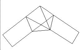
Here stand the pattern knot again. One should compare this freely woven window with the traditional (Celtic) alternating weave.

The pattern weave is not flat and it can be inscribed on the surface of a sphere or see as weaving between two spheres. It is curious that

almost always in decorative knots, the weaves are shown to be alternating. One reason for this is that a non-alternating weave may have a simpler alternating form. For example the pattern weave above is topologically equvalent to a simple trefoil knot.

Non minimal forms a knot can be interesting for their intrinsic geometry.

But note how quickly we are arriving at these patterns from the generation of a circle, of a distinction. There is an abstract level underlying all this where we note that the creation of the circle itself is an act of self-reference, the act of the drawing returning to itself.

The paradigm of a self-referential form is a form that reenters its own indicational space as in

You might interpret the reentrant form as an infinite descent of inclusions. Certainly the reentrant form is a precursor to the knots.

Instead of taking circularity out of the plane into three dimensional space, self-reference or reentrance takes the circularity into a spiral form that moves inward into a self-applied autonomy or self-producing structure. Both the knot and the reentrant form define themselves through a circularity.

An infinite nest of boxes certainly reenters its own indicational space and thereby becomes "knotted". This form of the knotting requires an excursion to infinity that is somehow related abstractly to the unfolding of the planar form into three dimensional space. At this point we return to the theme of the circularities of the Chinese five elements and their relationship with the very non-planar Petersen graph. The Petersen graph has in its own way a reentrant property that we will discuss in a later section of this essay.

Reentrance comes about through a duplicating operator. Let G denote this "Gremlin":

The gremlin acts on any form that it encounters by duplicating that form and putting the duplication into its interior space. Thus the gremlin is distinction that acts on other distinctions by duplicating them and transferring them from outer space to inner space. Incidentally, gremlins only get to act once. The distinction surrounding the duplicates is benign.

Now consider how a gremlin will act upon a gemlin! One gremlin will duplicate the other and place the duplicates inside its distinction. Inside the distinction there are now two interacting gremlins!

Thus the interaction of two gremlins reenters its own indicational space and we can write.

If you think of the two gremlins as an "inner sphere" and an "outer sphere", then the "knot" of the reentrance is produced by their interaction, and as the equation above shows, this knot IS the interaction of the two spheres. I like to think that this story about the interaction of the gremlins is what lies behind all of the geometric appearances of the weavings between two spheres. This is the structure of all mythologies of creation of heaven, earth and the creatures in between. This is the creation from polar opposites (the eaten and the eater) that are nevertheless the same and "they" are identical with their offspring.

Lets say this once more with symbols.

GA = F(AA) for any A.

Hence GG = F(GG) and so we see that

Two-fold interlocked action of duplication produces

infinite recursion.

Two-fold interlocked action of duplication produces

reentrance of indicational space.

Action of universe on itself to duplicate itself produces

knot of self-reference.

Formalism acting on itself is (k)not.

In the figure above I illustrate another approach to this formalism.

The gremlin is now a simple circle that has the property that it causes the internal duplication of any distinction placed inside it. That is, if you place an empty rectangle inside the circle then the result is a rectangle within a rectangle within the circle. In the case of a rectangle the process stops there. But if you place a circle in the circle, then the inner circle is replaced by a circle in a circle and the process continues forever. In notation, the change is to write

G(A) = F(A(A)) (F could be G itself). Then G(G) = F(G(G)).

This last version is closest to the geometry that we have been contemplating, since it is a generative process that is seeded by two concentric spheres and the result is a Godelian knot.

In fact, we have in this last version a significant variation of the orthodox version of the "Church-Curry Fixed Point Theorem".

The orthodox version goes:

Let G(A) = F(A(A)) for any A.

Then G(G) = F(G(G)).

Hence G(G) is a fixed point for F.

The variation goes:

Let G(A) = F(A(A)) for any A.

Let F = G.

Then G(A) = G(A(A)).

Once we let F=G, the process begins to spin an infinite sequence of forms.

G(A) = G(A(A)) = G(A(A)(A(A))) = G(A(A)(A(A))(A(A)(A(A)))) = ...

The geometry of this recursive process is illustrated below.

G being defined in terms of itself, acts as a catalyst promoting the generation of an infinite sequence of more and more complex forms.

In fact, from the figure above, the reader can see that the skeletons of these generated forms can be viewed as a sequence of sets. The empty box is an empty set, the box within a box is a set with one member, the empty box. The next set has two members consisting of the empty box and the box whose member is an empty box. Each succeeding set has one more member than the preceding set. This squence of sets (as sets) was discovered by John von Neumann as a method for creating represetative multiplicities within set theory.

Numbers are created from nothing but the act of forming a collection from previously created sets. This form of recursion does the collecting automatically.

Of course if would be good to see how such structures are related to the interaction of polyhedra in three dimensional space.

It is in fact easier to see how knots and links and weaves are related to circularities and self-reference since they are so close in formal structure. The next sections discusses these aspects.

IV. The Trefoil Knot, the Pentagon and the Golden Ratio

First we begin with an experiment that you can do with the trefoil knot and a strip of paper. Tie the strip into a trefoil and pull it gently tight and fold it so that you obtain a flat knot.

As you pull it tight with care a pentagon will appear!

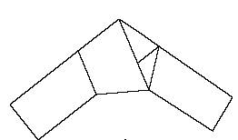
Now it is intuitively clear that this pentagonal form of the trefoil knot uses the least length of paper for a given width of paper (to make a flattened trefoil). At this writing, I do not have a proof of this

statement, but stand by!

What we can do is to determine the length to width ratio of the strip of paper obtained from this construction, by cutting the knot exactly along the edges of the pentagon.

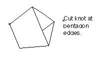
Then unfold this strip.

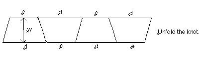
The lengths e and d that you see on this strip are the edge length e and the chord length d of the pentagon. To see this, contemplate the following two figures. We have that the length of the whole strip is L = 2(e+d).

First, here is the srtip folded back.

Here is a blown-up picture of the pentagon with the edge-length e, the chord d and the width of the strip w labeled. You can see from the previous picture that the width is indeed the length of a perpendicular dropped to the chord. It is also apparent from this diagram that W^{2} + (d-e)^{2}/4 = e^{2} (where a^{2} means "a squared"). Thus we can solve for the width W of the strip in terms of e and d. The result is

W = Sqrt(3 e^{2} - d^{2} + 2 ed)/2.

Thus, since L = 2(d+e), the ratio of length to width is

L/W = 4(d+e)/Sqrt(3 e^{2} - d^{2} + 2 ed)

= 4((d/e) +1)/Sqrt(3 - (d/e)^{2} + 2(d/e)).

Let F = d/e. Then we have

L/W = 4(F+1)/Sqrt(3 - F^{2} + 2F).

This is a formula for the length to width ratio of the flattened pentagonal trefoil knot. But now we use a classical fact about the pentagon.

FACT: The ratio F = d/e of the chord of a regular pentagon to its edge length is equal to the golden ratio. That is, F = (1 + Sqrt(5))/2 and

F^{2} = F + 1.

To see this fact, contemplate the following figure.

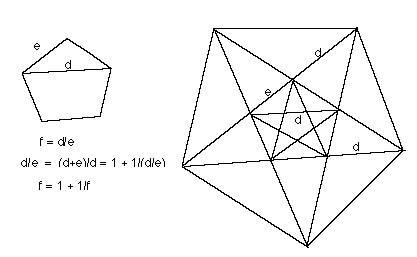
The small pentagon has its edge e and chord d labeled. We embed the small pentagon in the larger one and observe via a parallelogram and by similar triangles that

d/e = (d+e)/d (similar triangles).

Thus with F = d/e we have

d/e = 1 + e/d whence

F = 1 + 1/F.

This is sufficient to show that F is the golden ratio. Note how the golden ratio appears here through the way that a pentagon embeds in a pentagon, a pentagonal self-reference.

We conclude that

L/W = 4(F+1)/Sqrt(3 - F^{2} + 2F) = 4(F+1)/Sqrt(2 + F)

Thus

L/W = 4(F+1)/Sqrt(2+F).

This shows how the golden ratio appears crucially in this fundamental parameter associated with the trefoil knot.

Numerically, we find that

L/W = 5.5055276818846941528288383276435507181035973440326346534627030624763807750686919402638119724402807695804036548111386751892802062515920120151651883890946982137997852995080470479127188021558730989668039744257134892582786830818310791466934983280725762111661594340247094188738676759374984645289009953348098294865794745339707226530783308301329971259210594951174538320393858963073886494670463717651788969424799581801815247129118258205176981085866761468580327958439311118906154098770818806133886796185791615......

Quite a composition of fives!

It would be great to have a proof of the conjecture that L/W is indeed the minimum length to width ratio for a flattened trefoil.

More significantly, we would like to know if there is a relationship between this analysis and the properties of the trefoil as a geometric entity in three dimensional space. Specifically, I would like to know if there is a relationship between this flat geometry and the way in which Bob Gray has managed to fit the "pattern" trefoil on the surface of a rhombic triacontahedron. Here is his template for that fitting.

If you cut this figure out of paper and glue it into the three-dimensional object that it represents, you will have constructed a very nice pattern knot woven on the surface of a rhombic triacontahedron.

Here is Bob Gray's three dimensional visualization of this weaving.

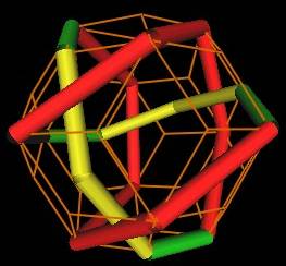
Is this three dimensional geometry related to the intrinsic flat golden ratio geometry of the trefoil knot?

V. Knots, Links, Circularities and a Weaving Calculus

The same diagrams that are used for drawings of knots and links can be used to illustrate the relationship of membership (for a non-standard version of set theory) by using the convention shown below.

In this convention each line has a label and the broken line is interpreted as passing underneath the unbroken line. If A is the label of the overcrossing line and B the label of the undercrossing line, then we say that "A is a member of B" and write A e B.

In order to begin the formalism of a set theory we need a notion of membership. This diagrammatic gives us the opportunity to depict various patterns of membership and to make a model that is topological in nature. We can use diagrams with or without free ends to depict these sets. For example

can represent the empty set, while

depicts both the empty set and the set whose only member is the empty set. Iteration of this idea produces a diagrammatic for the

von Neumann construction of sets with increasing finite cardinalities.

The knot diagrams afford the possibility to exhibit sets with strange properties, such as M, the set whose only member is itself.

Another phenomenon is mutuality such as A and B with each a member of the other: A = {B} and B={A}.

The linked sets are depicted by a topological link.

This version of set theory is closely related to the topology of knots and links if we understand the following diagram.

Here we have the sets A and B with A having B twice as a member.

Thus A is a multiset (many instances of identical members) and

must have a reduced representative in the set theory where each member of the reduced set occurs exactly once. In ordinary set theory, we reduce a multiset to a set by taking one representative copy of each member. Thus the reduced version of A would be

A'= {B} in the usual set theory. If, on the other hand, A and B are to be related to the topology of knots and links then we have to take into account that the diagram below is topologically equivalent to the one above.

Yet here we find that A is empty!

What saves the day is the "fermionic" convention for reducing a multiset to a set. In the fermionic convention, pairs of identicals

cancel to nothing so that { B,B, C } reduces to { C } while the

set consisting of three copies of B will reduce to one with a single copy of B. With the adoption of fermionic reduction, we are close to being able to state that topologically equivalent diagrams induce equivalent fermionic multi-sets. Set diagrams, under the fermionic convention are invariant under the following "Second Reidemeister Move":

Reidemeister proved in the 1920's that diagrams of knots and links

under the equivalence relation generated by the Reidemeister moves I, II and III (plus graphical equivalence in the plane) are the same as the topological equivalence classes of knots embedded in three dimensional space. Here is Reidemeister move III ( are representative version).

In the third Reidemeister move, one strand passes consecutively under (over) two other strands that themselves cross over each other. The strand that passes consecutively under (over) the other two strands can be moved as shown without affecting the topological type of the link. It is evident from this diagram that the third Reidemeister move does not affect the membership relations in the corresponding set.

Finally we get to the first Reidemeister move.

In order for our sets to be invariant under the first Reidemeister move, we need to make self-membership equivalent to non-self-membership. It is really quite innocuous to take self-membership lightly in this way. Thus we call a set a "knot-set" if it is obtained from a link or tangle diagrammatic description of a multiset with the equivalence relation generated by fermionic equivalence plus the added equivalence of self-membership and non-self membership.

If we keep self-membership and just use the fermionic equivalence, we call the resulting sets "fermionic sets". Knot sets and fermionic sets have topological diagrams that represent them.

The diagram above shows the sort of situation that is well-epressed by knot sets. Knot sets do not actually use knots. For example, the diagram of the trefoil knot T connotes the knot set

T = {T,T,T} = {T}

and this is in full knot sets equivalent to the empty set!

Now consider the diagram below.

We have for the multisets

A={B,B}

B={C,C}

C={A,A}.

A is over B, B is over C and C is over A.

This link is like the famous cycle Scissors, Paper, Stone!

Scissors cuts paper. Paper covers stone. Stone breaks scissors.

This link is often called the Borommean Rings and it is famous because it is indeed linked (no Reidemeister moves will unlink it). We will call it the Boro diagram.

Yet if you remove either A or B or C from the Borommean Rings, then the other two components are unlinked. For example, if we remove A, then B and C are unlinked.

What sort of knot set does the Boro diagram produce? Well, we cancle pairs of identicals and so the Boro diagram is equivalent to three empty sets. The topological linking of the Borommean Rings is not detected by their corresponding knot set.

It is interesting to try to generalize our language for linking so that the scissors, paper, stone property of the Borommean rings is seen to be the property that determines its linking. We will attempt this by

having one label per link component, just as in knot set theory. But we shall associate to each component an ordered list of the other components in terms of whether the given component is under or over the other component. If, as you traverse a component R you go under x, over y and under z, then we will write

R = UxOyUz. We can then see what the effect will be on these codes when we do the Reidemeister moves, and thereby obtain a language for studying linking that is more sophisticated than the knot set theory. For the Borromean Rings we have

A = OBUCOBUC

B = OCUAOCUA

C = OAUBOAUB.

Now the repetitions are separated by other symbol strings and we can begin to see that there will be no way to undo these symbols the way we cancelled the repetitions in the knot sets for the Borommean Rings. Of course, a careful analysis is called for. We must begin by lookking at the effects on these symbol sequences by the Reidemeister moves.

In the case of the first Reidemeister move, we see that we can, in the string corresponding to a label A, insert or remove an occurrence of

OAUA or UAOA.

In the case of the second Reideimeister move, we see that we can still cancel consecutive occurences of a symbol from a string but that we need two overs in one string matched by two unders in the other as shown above.

Finally, we see in the third Reidemeister move, that the pattern of triangle involvement is replaced by swithching the order of encounters along each line.

Call the formal language of symbol strings with these rules the Weaving Calculus.

The Weaving Caclculus is the closest structure to the knot sets that contains more topology. I conjecture that the Borommean rings are non-trivial in this string language. The reader may enjoy proving that all knots (one component) have corresponding symbol strings that can be unravelled. Knots are not detected by the Weaving Calculus.

VI. Euler's Formula

The last sections have contained a mixture of speculations, mythology and new mathematics. In this section I will review a piece of mathematics first discovered by Leonhard Euler in the 18th century. This mathematics is old but it is a fresh as if newly minted in the 21st century.

Euler proved that if a connected planar graph has V nodes, E edges and F faces, then V-E+F = 2.

With the help of this result one has an entirely new approach to the Euclidean classification of the regular solids, and a corresponding approach to regular and semi-regular polyhedra. We will continue this section in the next installment of these notes.