The Lorenz attractor (AKA the Lorenz butterfly) is generated by a set of differential equations which model a simple system of convective flow (i.e. motion induced by heat). In a paper published in 1963, Edward Lorenz demonstrated that this system exhibits chaotic behavior when the physical parameters are appropriately chosen.
The Lorenz system is deterministic, which means that if you know the exact starting values of your variables then in theory you can determine their future values as they change with time. Lorenz demonstrated that if you begin this model by choosing some values for x, y, and z, and then do it again with just slightly different values, then you will quickly arrive at fundamentally different results. In real life you can never know the exact value of any physical measurement, although you can get close (imagine measuring the temperature at O'Hare Airport at 3:15 AM). See the problem? With these results, Lorenz shocked the mathematical and scientific community by showing that a seemingly nice system of equations could defy conventional methods of prediction. This is called chaos, and its implications are far-reaching, especially in the field of weather prediction.
Below are some images of the Lorenz attractor that I created in 2008 at the MSRI Climate Change Summer School.
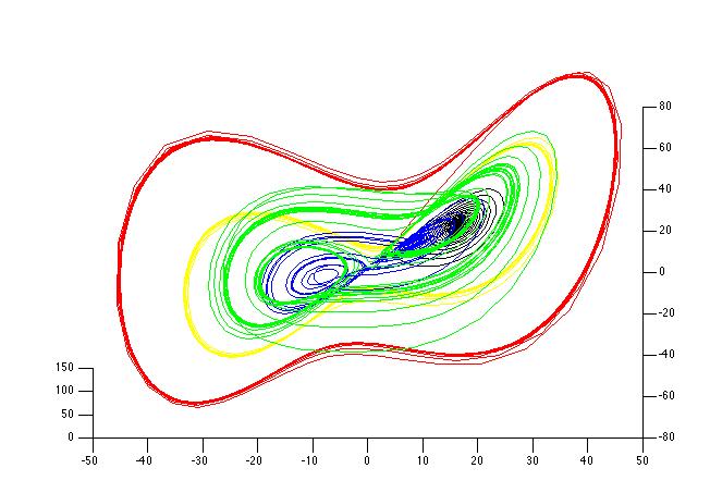
This is what the standard Lorenz butterfly looks like:
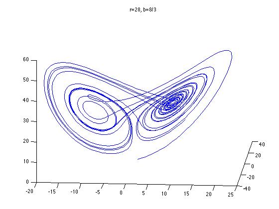
Notice the two "wings" of the butterfly; these correspond to two different sets of physical behavior of the system. A point on this graph represents a particular physical state, and the blue curve is the path followed by such a point during a finite period of time. Notice how the curve spirals around on one wing a few times before switching to the other wing.
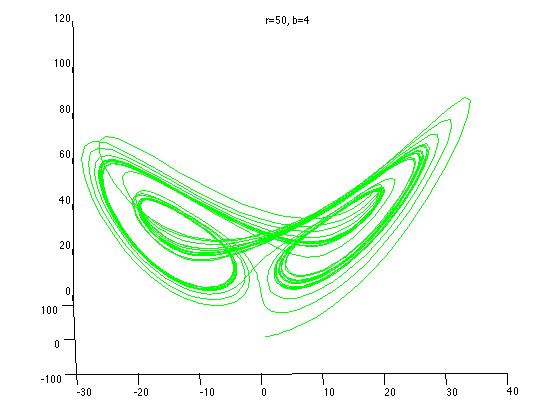
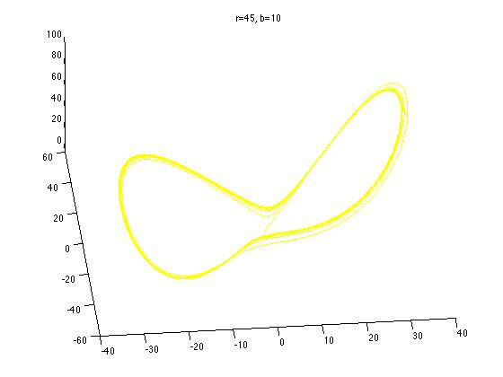
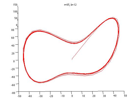
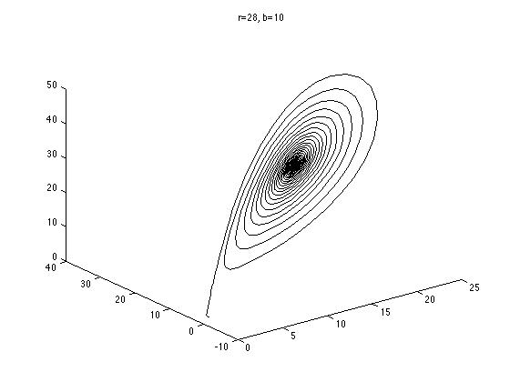
By varying the physical parameters of the Lorenz system, one can get quite different results:
[Disclaimer: An error was pointed out to me that some of these plots are incorrect, based on the too-simple time integrator used (Forward Euler method). I would recommend using a small timestep (dt=0.001) or implementing a more sophisticated solver such as Runge-Kutta 4th order. The code has been updated, but the plots haven't yet been updated. Thanks to https://www.drupal.org/u/pol]
As a way to quantify the different behaviors, I chose to focus on the frequency with which the model switched states, from one "wing" to the other. By running a series of simulations with different parameters, I arrived at the following set of results:
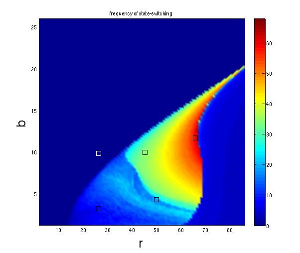
This colors on this graph represent the frequency of state-switching for each set of parameters (r,b).
The five points marked on the above graph correspond to the five different Lorenz systems whose graphs are plotted above. All together now:
Here's what the equations look like:
x' = σ(y - x)
y' = x(r - z) - y
z' = xy - bz
The state variables are x, y, and z. The rate at which x is changing is denoted by x'. The physical parameters are σ, r, and b.
In my examples, (x,y,z) begins near (5,5,5) and σ=10.
Here is some MATLAB code that I used. DISCLAIMER: The code is old, sloppy, and poorly documented. Sorry. Analogous Python code can be found here: http://matplotlib.org/examples/mplot3d/lorenz_attractor.html
Quick tip: To generate the first plot, open Octave or Matlab in a directory containing the files "func_LorenzEuler.m" and "easylorenzplot.m", then run the command "easylorenzplot(10,28,8/3,5,5,5,'b')".
mylorenz.m
mylorenz2.m
easylorenzplot.m
func_LorenzEuler.m
func_noisyLorenzEuler.m
[A more proper approach would be to define a function such as in "func_LorenzEuler.m" and use it with lsode (Octave) or ode45 (Matlab).]
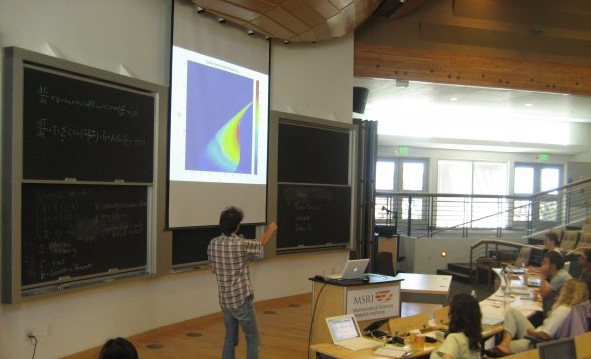
Oh and here's a picture of me presenting these results at MSRI during the 2008 climate change summer school:
New movie here! http://youtu.be/5mI8dxs6-BY
( back to main page )