Increment-and-Fix Aposteriori Step Control
An artificial-parameter homotopy to solve
with the total degree start system
uses a random complex constant \(\gamma\) in
where \(t\) is an artificial parameter to define the deformation of the start system into the target system.
During the continuation, a predictor-corrector method is applied. The predictor advances the value of \(t\), predicts the corresponding solution for the new value of \(t\), and then fixes the value of \(t\) in the corrector stage. Because \(t\) is fixed during the corrector stage, this type of continuation is called increment-and-fix continuation.
An aposteriori step size control algorithm uses the performance of the corrector to determine the step size for the continuation parameter \(t\).
Let us first define the target and start system for the running example.
target = ['x^2 + 4*y^2 - 4;', '2*y^2 - x;']
A start system based on the total degree is constructed.
from phcpy.starters import total_degree_start_system
start, startsols = total_degree_start_system(target)
The len(startsols) returns 4 and thus we have 4 paths.
For deterministic runs, we set the seed of the random number generators:
from phcpy.dimension import set_seed
set_seed(2024)
let the path trackers run
To run the path trackers in double precision:
from phcpy.trackers import double_track
and then call double_track as follows:
gamma, sols = double_track(target, start, startsols)
By default, double_track will generate a random \(gamma\)
and return the generated value. This value can then be used in a second run.
To print the solutions, execute the following code:
for (idx, sol) in enumerate(sols):
    print('Solution', idx+1, ':')
    print(sol)
and what is then printed is
Solution 1 :
t :  1.00000000000000E+00   0.00000000000000E+00
m : 1
the solution for t :
 x :  1.23606797749979E+00   1.63132611699963E-55
 y :  7.86151377757423E-01  -1.62115537155392E-56
== err :  1.383E-16 = rco :  1.998E-01 = res :  2.220E-16 =
Solution 2 :
t :  1.00000000000000E+00   0.00000000000000E+00
m : 1
the solution for t :
 x :  1.23606797749979E+00   1.63132611699963E-55
 y : -7.86151377757423E-01   1.62115537155392E-56
== err :  1.383E-16 = rco :  1.998E-01 = res :  2.220E-16 =
Solution 3 :
t :  1.00000000000000E+00   0.00000000000000E+00
m : 1
the solution for t :
 x : -3.23606797749979E+00   1.06910588403688E-50
 y : -5.34552942018439E-51  -1.27201964951407E+00
== err :  7.222E-35 = rco :  1.079E-01 = res :  3.130E-50 =
Solution 4 :
t :  1.00000000000000E+00   0.00000000000000E+00
m : 1
the solution for t :
 x : -3.23606797749979E+00   1.06910588403688E-50
 y :  5.34552942018439E-51   1.27201964951407E+00
"== err :  7.222E-35 = rco :  1.079E-01 = res :  3.130E-50 =
Of the four solutions, observe that two are complex conjugated. The start solutions are all real and if the \(\gamma\) would have been real as well (with a zero imaginary part), then the transition from the real start solutions to the solutions with nonzero imaginary parts would not have been possible.
Suppose we would want to recompute the first path in quad double precision.
from phcpy.trackers import quad_double_track
Even if we track only one path, the start solution must be given
in a list of one element.
Observe that we use the same value of gamma as before.
gamma, qdsol = quad_double_track(target, start, [startsols[0]], gamma=gamma)
print(qdsol[0])
and what is printed is
t : 1.0000000000000000000000000000000000000000000000000000000000000000E+00      0.0000000000000000000000000000000000000000000000000000000000000000E+00
m : 1
the solution for t :
 x : 1.2360679774997896964091736687116429937402734744492267964203321508E+00      3.5725407585478398168188068938476209257268222381106725605357869223E-29
 y : 7.8615137775742328606955858582272987880739633619149401238232806827E-01      1.9775278344660286732240368562738254609143580079378403594856065932E-29
== err :  1.850E-14 = rco :  1.998E-01 = res :  3.884E-28 =
Observe that the values for the forward and backward error,
the err and res respectively, are still rather large
for quad double precision. For this example, we could as well
run a couple of extra steps of Newton’s method, but suppose
that we want to track the complete path with much smaller tolerances.
tuning tolerances of the path trackers
Let us redo the last run, but now with much smaller tolerances on the corrector. The output of
from phcpy.trackers import write_parameters
write_parameters()
is
GLOBAL MONITOR :
  1. the condition of the homotopy           : 0
  2. number of paths tracked simultaneously  : 1
  3. maximum number of steps along a path    : 500
  4. distance from target to start end game  : 1.000e-01
  5. order of extrapolator in end game       : 0
  6. maximum number of re-runs               : 1
STEP CONTROL (PREDICTOR) :                    along path : end game
  7: 8. type ( x:Cub,t:Rea ):( x:Cub,t:Rea ) : 8         : 8
  9:10. minimum step size                    : 1.000e-06 : 1.000e-08
 11:12. maximum step size                    : 1.000e-01 : 1.000e-02
 13:14. reduction factor for step size       : 7.000e-01 : 5.000e-01
 15:16. expansion factor for step size       : 1.250e+00 : 1.100e+00
 17:18. expansion threshold                  : 1         : 3
PATH CLOSENESS (CORRECTOR) :                  along path : end game
 19:20. maximum number of iterations         : 3         : 3
 21:22. relative precision for residuals     : 1.000e-09 : 1.000e-11
 23:24. absolute precision for residuals     : 1.000e-09 : 1.000e-11
 25:26. relative precision for corrections   : 1.000e-09 : 1.000e-11
 27:28. absolute precision for corrections   : 1.000e-09 : 1.000e-11
SOLUTION TOLERANCES :                         along path : end game,
 29:30. inverse condition of Jacobian        : 1.000e-04 : 1.000e-12
 31:32. clustering of solutions              : 1.000e-04 : 1.000e-12
 33:34. solution at infinity                 : 1.000e+08 : 1.000e+12
Let us tune of the parameters of the corrector.
To set the tolerance for the relative precision for the residuals
along the path to 1.0e-32, the parameter at position 21
has to be set, as follows:
set_parameter_value(21, 1.0e-32)
and then running write_parameters() again will show
21:22. relative precision for residuals : 1.000e-32 : 1.000e-11
as the line that has changed.
For this problem, the difference between absolute and relative
does not matter, and neither does the difference between
the residuals and corrections, as the paths are well conditioned.
Along the path, we set the tolerance to 1.0e-32
and at the end to 1.0e-48.
for idx in [23, 25, 27]:
    set_parameter_value(idx, 1.0e-32)
for idx in [22, 24, 26, 28]:
    set_parameter_value(idx, 1.0e-48)
Now we rerun the first path once more.
gamma, qdsol = quad_double_track(target, start, [startsols[0]], gamma=gamma)
print(qdsol[0])
and what is printed is
t : 1.0000000000000000000000000000000000000000000000000000000000000000E+00      0.0000000000000000000000000000000000000000000000000000000000000000E+00
m : 1
the solution for t :
 x : 1.2360679774997896964091736687312762354406183596115257242708972454E+00      -5.2497200000892523553940877198954046619454940726389357724082489942E-135
 y : 7.8615137775742328606955858584295892952312205783772323766490197012E-01      -5.8637627799330186773963784283091100994566589683500740754044455987E-133
== err :  3.218E-66 = rco :  1.998E-01 = res :  2.018E-65 =
Observe that the values of err and res
(forward and backward error respectively) are much smaller than before,
very close to the quad double precision.
For the experiments in the next section, the values of the continuation parameters must be reset to their defaults.
from phcpy.trackers import autotune_parameters
autotune_parameters(0, 14)
The 0 stands for the default and 14 to take into account
the 14 decimal places of precision.
a step-by-step path tracker
When we run a path tracker, or let a path tracker run, then the path tracker has the control of the order of execution. In a step-by-step path tracker, we can ask the path tracker for the next point of the path, which is useful to plot the points along a path.
from phcpy.trackers import initialize_double_tracker
from phcpy.trackers import initialize_double_solution
from phcpy.trackers import next_double_solution
The initialization of the tracker is separate from the initialization of a solution, as the same homotopy is used to track all paths.
initialize_double_tracker(target, start)
The first parameter in initialize_double_solution
is the number of variables, which equals the number
of polynomials in the target system.
initialize_double_solution(len(target), startsols[0])
The first step
- ::
nextsol = next_double_solution() print(nextsol)
shows
t :  1.00000000000000E-01   0.00000000000000E+00
m : 1
the solution for t :
 x :  9.96326698649568E-01   4.70406409720798E-03
 y :  9.96408257454631E-01   4.95315220446915E-03
== err :  2.375E-05 = rco :  1.000E+00 = res :  3.619E-10 =
and then the second step
nextsol = next_double_solution()
print(nextsol)
gives
t :  2.00000000000000E-01   0.00000000000000E+00
m : 1
the solution for t :
 x :  9.79864035891029E-01   1.70985015865591E-02
 y :  9.81181263858417E-01   2.32157127720825E-02
== err :  1.679E-08 = rco :  1.000E+00 = res :  2.760E-16 =
In a loop, we want to stop as soon as the value of t passes 1.0.
To get the value of t out of a solution string,
we convert the string into a dictionary, as done below:
from phcpy.solutions import strsol2dict
dictsol = strsol2dict(nextsol)
dictsol['t']
shows
(0.2+0j)
In the code cell below, the loop continues
calling next_double_solution until the value
of the continuation parameter is less than 1.0.
The real part and imaginary part of the gamma constant
are set to the same value of gamma as in the first run.
initialize_double_tracker(target, start, fixedgamma=False, \
                          regamma=gamma.real, imgamma=gamma.imag)
initialize_double_solution(len(target), startsols[0])
tval = 0.0
path = [startsols[0]]
while tval < 1.0:
    nextsol = next_double_solution()
    dictsol = strsol2dict(nextsol)
    tval = dictsol['t'].real
    path.append(nextsol)
All values of the x-coordinates of all points on the path:
(1+0j)
(0.996326698649568+0.00470406409720798j)
(0.979864035891029+0.0170985015865591j)
(0.943788099865787+0.00964655321202273j)
(0.950990471736517-0.0674242744055464j)
(1.06214893672862-0.108107883550403j)
(1.15606754413692-0.0765694315601522j)
(1.20399680236398-0.0383121382228797j)
(1.2254591757779-0.0141573296657659j)
(1.23400325696781-0.00289013787311083j)
(1.23606797749301-4.13424477147656e-11j)
are obtained with
for sol in path:
    print(strsol2dict(sol)['x'])
To put the real parts of the x-coordinates in a list:
xre = [strsol2dict(sol)['x'].real for sol in path]
and likewise, the imaginary parts of the x-coordinates and the two parts of the y-coordinates are set by the code below:
xim = [strsol2dict(sol)['x'].imag for sol in path]
yre = [strsol2dict(sol)['y'].real for sol in path]
yim = [strsol2dict(sol)['y'].imag for sol in path]
Let us plot the coordinates of this first solution path.
import matplotlib.pyplot as plt
The coordinates of the solution path are then plotted in Fig. 20 as follows.
fig, axs = plt.subplots(1, 2, constrained_layout=True)
fig.suptitle('the coordinates of one solution path')
axs[0].set_title('x coordinates')
axs[0].set_xlabel('real part')
axs[0].set_ylabel('imaginary part')
axs[0].set_xlim(min(xre)-0.1, max(xre)+0.1)
axs[0].set_ylim(min(xim)-0.025, max(xim)+0.025)
dots, = axs[0].plot(xre,xim,'r-')
dots, = axs[0].plot(xre,xim,'ro')
axs[1].set_title('y coordinates')
axs[1].set_xlabel('real part')
axs[1].set_ylabel('imaginary part')
axs[1].set_xlim(min(yre)-0.1, max(yre)+0.1)
axs[1].set_ylim(min(yim)-0.025, max(yim)+0.025)
dots, = axs[1].plot(yre,yim,'r-')
dots, = axs[1].plot(yre,yim,'ro')
plt.savefig('incfixaposteriorifig1')
plt.show()
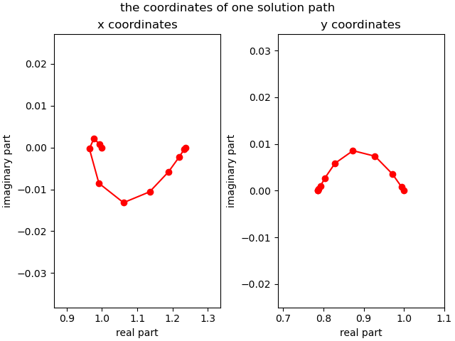
Fig. 20 The coordinates of one solution path.
Why do the paths in such a simple homotopy curve so much?