Recursive Drawings¶

Applying simple rules recursively, we can draw remarkable pictures. For recursive images, the design of a GUI with canvas, scale, and button, can always be very similar. The action is defined by a callback function. We start with simple drawings, such as a regular n-gon or a Cantor set, before making more complicated plots. The more advanced mathematical computations are defined in separate functions, isolating the complexity to some critical spots.

A Regular n-Gon¶

For starters, let us draw a regular n-gon, as shown in Fig. 16.

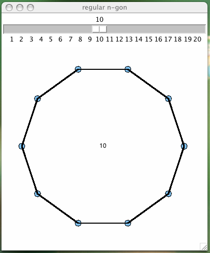
Fig. 16 A multigon drawn on a Tkinter canvas.

The structure of the GUI to produce Fig. 16 is listed below. In the design of the class MultiGon, we write the doc strings first.

class MultiGon(object):
    """
    GUI to draw a regular n-gon on canvas.
    """
    def __init__(self, wdw):
        """
        Determines the layout of the GUI.
        """
    def draw_gon(self, val):
        """
        Draws a regular n-gon.
        """
def main():
    """
    Instantiates the GUI object
    and launches the main event loop.
    """

The layout of the GUI consists of a horizontal scale, for the user to determine the number n of vertices of the n-gon. The cancase is the second widget of the GUI, as defined in the function below.

from tkinter import Tk, IntVar, Scale, Canvas, ALL

def __init__(self, wdw):
    """
    Determines the layout of the GUI.
    """
    wdw.title('regular n-gon')
    self.dim = 400
    self.ngn = IntVar()
    self.scl = Scale(wdw, orient='horizontal', \
        from_=1, to=20, tickinterval=1, \
        length=self.dim, variable=self.ngn, \
        command=self.draw_gon)
    self.scl.set(10)
    self.scl.grid(row=0, column=0)
    self.cnv = Canvas(wdw, width=self.dim, \
        height=self.dim, bg='white')
    self.cnv.grid(row=1, column=0)

The Scale triggers the command draw_gon() and determines the data attribute ngn of a MultiGon object. The second argument val is the value for ngn passed to draw_gon() via the Scale.

def draw_gon(self, val):
    """
    Draws a regular n-gon.
    """
    xctr = self.dim/2
    yctr = self.dim/2
    radius = 0.4*self.dim
    self.cnv.delete(ALL)
    self.cnv.create_text(xctr, yctr, text=val, tags="text")
    ngn = int(val)

The value val is passed as a string. Therefore, we convert to an integer in the statement ngn = int(val). After obtaining the value for n, the method can draw the vertices and the edges between the vertices. In a regular n-gon, all n points lie on a circle, equispaced using the angle $2 \pi/n$. Therefore we add the following import statement.

from math import cos, sin, pi

Then the code for the method draw_gon() continues.

# the method draw_gon() continued ...
    pts = []
    for i in range(0, ngn):
        xpt = xctr + radius*cos(2*i*pi/ngn)
        ypt = yctr + radius*sin(2*i*pi/ngn)
        self.cnv.create_oval(xpt-6, ypt-6, xpt+6, ypt+6, \
            width=1, outline='black', fill='SkyBlue2', \
            tags="dot")
        pts.append((xpt, ypt))
    for i in range(0, ngn-1):
        self.cnv.create_line(pts[i][0], pts[i][1], \
            pts[i+1][0], pts[i+1][1], width=2)
    self.cnv.create_line(pts[ngn-1][0], pts[ngn-1][1], \
        pts[0][0], pts[0][1], width=2)

We will apply the template of the multigon to draw a sequence of recursive images, starting with the Cantor set in Fig. 17. This figure is then generalized into the Koch curve, in Fig. 18 and the Koch flake in Fig. 19. Two other self similar images are the Sierpinski gasket, shown in Fig. 20 and Hilbert curves, drawn in Fig. 21.

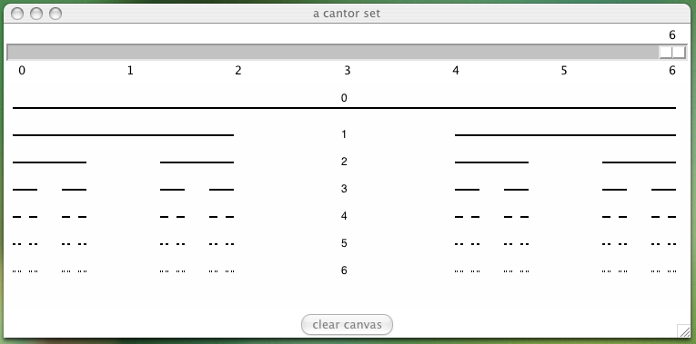
Fig. 17 A Cantor set on a Tkinter canvas.

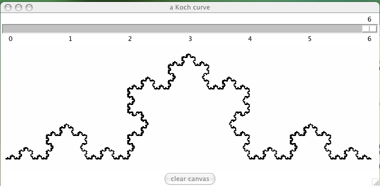
Fig. 18 A Koch curve on a Tkinter canvas.

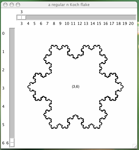
Fig. 19 A Koch flake on a Tkinter canvas.

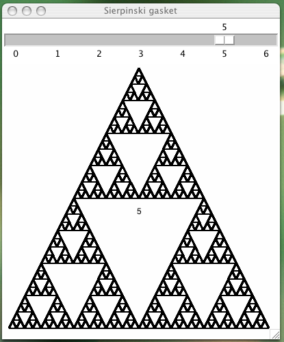
Fig. 20 A Sierpinski gasket on a Tkinter canvas.

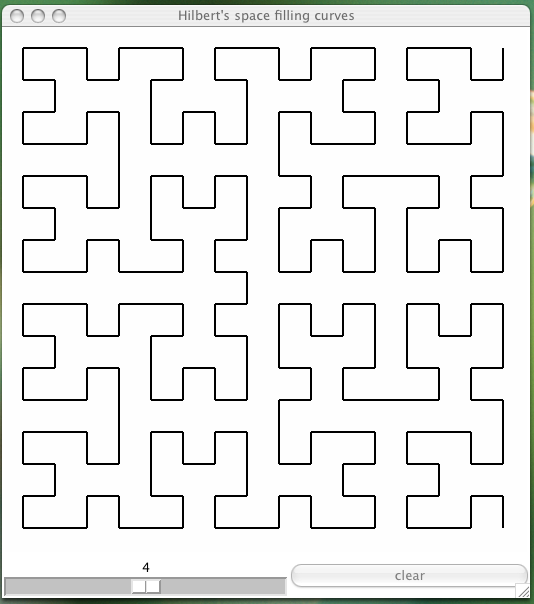
Fig. 21 A GUI for Hilbert curves.

The Cantor set is defined by three rules:

Take the interval~$[0,1]$,
Remove the middle part third of the interval.
Repeat rule textcolor{blue}{2} on the first and third part.

The Cantor set is infinite, to visualize at level $n$:

for $n = 0$: start at $[0,1]$,
for $n > 0$: apply the rule $2 n$ times.

In our definition of the class CantorSet, we will write the doc strings first of the methods.

class CantorSet(object):
    """
    GUI to draw a Cantor set on canvas.
    """
    def __init__(self, wdw, N):
        """
        A Cantor set with N levels.
        """
    def cantor(self, lft, rgt, hgt, txt, lvl):
        """
        Draws a line from lft to rgt, at height hgt,
        txt is a string, int(txt) equals the number
        of times the middle third must be removed,
        lvl is the level of recursion.
        """
    def draw_set(self, val):
        """
        Draws a Cantor set.
        """

The constructor of the class defines the layout of the GUI.

def __init__(self, wdw, N):
    """
    A Cantor set with N levels.
    """
    wdw.title('a cantor set')
    self.dim = 3**N+20
    self.nsc = IntVar()
    self.scl = Scale(wdw, orient='horizontal', \
        from_=0, to=N, tickinterval=1, length=self.dim, \
        variable=self.nsc, command=self.draw_set)
    self.scl.grid(row=0, column=0)
    self.scl.set(0)
    self.cnv = Canvas(wdw, width=self.dim, \
        height=self.dim/3, bg='white')
    self.cnv.grid(row=1, column=0)
    self.btt = Button(wdw, text="clear canvas", \
        command=self.clear_canvas)
    self.btt.grid(row=2, column=0)

The method clear_canvas() is triggered by the button. Its definition is below.

def clear_canvas(self):
    """
    Clears the entire canvas.
    """
    self.cnv.delete(ALL)

The method draw_set() is triggered by the scale. Its definition is below.

def draw_set(self, val):
    """
    Draws a Cantor set.
    """
    nbr = int(val)
    self.cantor(10, self.dim-10, 30, val, nbr)

The method cantor() is recursive. In designing a recursive function, more than half of the work goes into defining the right parameters.

def cantor(self, lft, rgt, hgt, txt, lvl):
    """
    Draws a line from lft to rgt, at height hgt;
    txt is a string, int(txt) equals the number
    of times the middle third must be removed;
    lvl is the level of recursion.
    """

The parameters lft, rgt, and hgt define the line segment from (lft, hgt) to (rgt, hgt). The parameter txt is the value passed via the Scale, as text string, txt is also put on Canvas.

The most important parameter is lvl. Initially: lvl = int(txt). With every recursive call, lvl is decremented by 1. The lvl in cantor(self, lft, rgt, hgt, txt, lvl) controls the recursion.

At lvl = 0, the line segment from (lft, hgt) to (rgt, hgt) is drawn.
For lvl > 0, we compute left and right limit of the middle third of [lft, rgt], respectively denoted by nlf and nrg as

\[\begin{split}\begin{array}{c} {\tt nlf} = {\tt lft} + ({\tt rgt}-{\tt lft})/3 = (2 {\tt lft} + {\tt rgt}) / 3 \\ {\tt nrg} = {\tt rgt} = ({\tt rgt}-{\tt lft})/3 = ({\tt lft} + 2{\tt rgt}) / 3 \end{array}\end{split}\]

Then we make two recursive calls:

self.cantor(lft, nlf, hgt+30, txt, lvl-1)
self.cantor(nrg, rgt, hgt+30, txt, lvl-1)

The code for the method cantor() is below:

def cantor(self, lft, rgt, hgt, txt, lvl):
    """
    Draws a line from lft to rgt, at height hgt;
    txt is a string, int(txt) equals the number
    of times the middle third must be removed;
    lvl is the level of recursion.
    """
    if lvl == 0:           # draw line segment
        self.cnv.create_line(lft, hgt, rgt, hgt, width=2)
    else:
        nlf = (2*lft+rgt)/3
        nrg = (lft+2*rgt)/3
        self.cantor(lft, nlf, hgt+30, txt, lvl-1)
        self.cantor(nrg, rgt, hgt+30, txt, lvl-1)
    if lvl == int(txt):      # put text string
        xctr = self.dim/2
        if txt == '0':
            self.cnv.create_text(xctr, hgt-10, text=txt)
        else:
            self.cnv.create_text(xctr, hgt+lvl*30, \
                text=txt)

The Koch curve is a Cantor set where the removed middle third of the interval is replaced by a wedge. The top of the wedge is above the midpoint of the removed middle interval. The slopes of the wedge make an angle of 60 degrees with respect to the rest of the line segment. To visualize a Koch curve at level $n$:

For $n = 0$: start at [0,1].
For $n > 0$: make wedges $n$ times.

In developing the class for the GUI, we write the doc strings of the methods in the class KochCurve first.

class KochCurve(object):
    """
    GUI to draw a Koch curve on canvas.
    """
    def __init__(self, wdw, N):
        """
        A Koch curve with N levels.
        """
    def koch(self, left, right, k):
        """
        A Koch curve from left to right with k levels.
        """
    def draw_curve(self, val):
        """
        Draws a Koch curve.
        """

The constructor defines the layout of the GUI, as defined below. Our GUI has a scale, canvas, and button.

def __init__(self, wdw, N):
    """
    A Koch curve with N levels.
    """
    wdw.title('a Koch curve')
    self.dim = 3**N+20
    self.nvr = IntVar()
    self.scl = Scale(wdw, orient='horizontal', \
        from_=0, to=N, tickinterval=1, \
        length=self.dim, variable=self.nvr, \
        command=self.draw_curve)
    self.scl.set(0)
    self.scl.grid(row=0, column=0)
    self.cnv = Canvas(wdw, width=self.dim, \
        height=self.dim/3, bg='white')
    self.cnv.grid(row=1, column=0)
    self.btt = Button(wdw, text="clear canvas", \
        command=self.clear_canvas)
    self.btt.grid(row=2, column=0)

The method clear_canvas() is triggered by a button. Its definition is below.

def clear_canvas(self):
    """
    Clears the entire canvas.
    """
    self.cnv.delete(ALL)

The method draw_curve() is activated by a scale. Its definition is below.

def draw_curve(self, val):
    """
    Draws a Koch curve.
    """
    nbr = int(val)
    left = (10, self.dim/3-20)
    right = (self.dim-10, self.dim/3-20)
    self.koch(left, right, nbr)

The method koch() is recursive, to draw a Koch curve of nbr levels from left to right. The parameter nbr in koch(left, right, nbr) controls the recursion.

For nbr = 0, the line segment from left to right is drawn.
For nbr > 0, we compute left nlf, right nrg, and midpoint mid of the middle third of line segment.

Now we fill the middle with a wedge. The edges of the wedge make an angle of 60 degrees. Then the height is $\sin(\frac{\pi}{3}) = \frac{\sqrt{3}}{2}$, multiplied with one third of the length of the segment.

The peak of the wedge is relative to the size of the interval and the position of the midpoint mid:

\[\begin{split}\begin{array}{l} {\tt top} = (\frac{\sqrt{3}}{6} ({\tt left}[1]-{\tt right}[1]), \frac{\sqrt{3}}{6} ({\tt right}[0]-{\tt left}[0])), \\ \\ {\tt peak} = ({\tt mid}[0]-{\tt top}[0],{\tt mid}[1]-{\tt top}[1]) \end{array}\end{split}\]

Recall that on the canvas: (0,0) is at the topmost left corner. The code for the method koch() is listed below.

def koch(self, left, right, k):
    """
    A Koch curve from left to right with k levels.
    """
    if k == 0:
        self.cnv.create_line(left[0], left[1], \
           right[0], right[1], width=2)
    else:
        nlf = ((2*left[0]+right[0])/3.0, (2*left[1]+right[1])/3.0)
        nrg = ((left[0]+2*right[0])/3.0, (left[1]+2*right[1])/3.0)
        mid = ((left[0]+right[0])/2.0, (left[1]+right[1])/2.0)
        ratio = sqrt(3)/6
        top = (ratio*(left[1]-right[1]), ratio*(right[0]-left[0]))
        peak = (mid[0]-top[0], mid[1]-top[1])
        self.koch(left, nlf, k-1)
        self.koch(nlf, peak, k-1)
        self.koch(peak, nrg, k-1)
        self.koch(nrg, right, k-1)

In the development of the GUI for the Koch flake, we write the doc strings of the class KochFlake first.

class KochFlake(object):
    """
    GUI to draw a Koch flake canvas.
    """
    def __init__(self, wdw):
        """
        Determines the layout of the GUI.
        """
    def koch(self, left, right, k):
        """
        A Koch flake from left to right with k levels.
        """
    def draw_flake(self, val):
        """
        Draws a regular Koch flake.
        """

The scales of the GUI are defined by the constructor, defined below.

def __init__(self, wdw):

    self.nbr = IntVar()
    self.k = IntVar()
    self.scn = Scale(wdw, orient='horizontal', \
        from_=3, to=20, tickinterval=1, \
        length=self.dim, variable=self.nbr, \
        command=self.draw_flake)
    self.scn.set(10)
    self.scn.grid(row=0, column=1)
    self.sck = Scale(wdw, orient='vertical', \
        from_=0, to=6, tickinterval=1,\
        length=self.dim, variable=self.k,\
        command=self.draw_flake)
    self.sck.set(0)
    self.sck.grid(row=1, column=0)

The code for the method draw_flake() follows.

def draw_flake(self, val):
    """
    Draws a regular Koch flake.
    """
    (xctr, yctr) = (self.dim/2, self.dim/2)
    radius = 0.4*self.dim
    self.cnv.delete(ALL)
    nbr = self.nbr.get()
    k = self.k.get()
    txt = '(' + str(nbr) + ',' + str(k) + ')'
    self.cnv.create_text(xctr, yctr, text=txt, tags="text")
    pts = []
    for i in range(0, nbr):
        xpt = xctr + radius*cos(2*i*pi/nbr)
        ypt = yctr + radius*sin(2*i*pi/nbr)
        pts.append((xpt, ypt))
    for i in range(0, nbr-1):
        self.koch(pts[i], pts[i+1], k)
    self.koch(pts[nbr-1], pts[0], k)

Space Filling Curves and L-systems¶

The first three Hilbert curves are shown in Fig. 22.

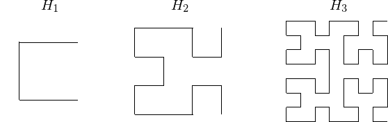
Fig. 22 The first three Hilbert curves.

The recursion is determined by the application of four types of moves, labeled A, B, C, and D in Fig. 23.

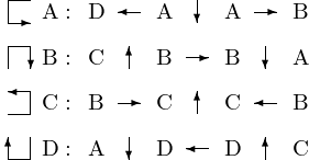
Fig. 23 Four types of moves in the recursion to make Hilbert curves.

In the development of the GUI for the Hilbert curves, we write the doc string first:

class Hilbert:
    """
    GUI for Hilbert's space filling curves.
    """
    def __init__(self,wdw,dimension):
        """
        Defines a canvas, buttons, and scale.
        """
    def plot(self, nxp, nyp):
        """
        Plots a line for the current position
        to the new coordinates (nxp, nyp), and
        sets the current position to (nxp, nyp).
        """
    def draw(self, val):
        """
        Draws the Hilbert curve on canvas.
        """

Then for each move in Fig. 23 we have a method. Their doc strings are listed below.

def amove(self, k):
    """
    Turns counterclockwise from up right to down right.
    """
def bmove(self, k):
    """
    Turns clockwise from down left to down right.
    """
def cmove(self, k):
    """
    Turns counterclockwise from down left to up left.
    """
def dmove(self, k):
    """
    Turns clockwise from up right to up left.
    """

The basic method plot() is defined below.

def plot(self, nxp, nyp):
    """
    Plots a line for the current position
    to the new coordinates (nxp, nyp), and sets
    the current position to (nxp, nyp).
    """
    self.cnv.create_line(self.xpt, self.ypt, \
        nxp, nyp, width=2)
    self.xpt = nxp
    self.ypt = nyp

The top level method is draw(), given next.

def draw(self, val):
    """
    Draws the Hilbert curve on canvas.
    """
    nbr = int(val)
    self.hgt = self.dim/2**nbr
    self.ypt = 5 + self.dim - self.hgt/2
    self.xpt = self.ypt
    self.amove(nbr)

The move A (see Fig. 23) is defined in the method amove().

def amove(self, k):
    """
    Turns counterclockwise from up right to down right.
    """
    if k > 0:
        self.dmove(k-1)
        self.plot(self.xpt - self.hgt, self.ypt)
        self.amove(k-1)
        self.plot(self.xpt, self.ypt - self.hgt)
        self.amove(k-1)
        self.plot(self.xpt + self.hgt, self.ypt)
        self.bmove(k-1)

The move B (see Fig. 23) is defined in the method bmove().

def bmove(self, k):
    """
    Turns clockwise from down left to down right.
    """
    if k > 0:
        self.cmove(k-1)
        self.plot(self.xpt, self.ypt + self.hgt)
        self.bmove(k-1)
        self.plot(self.xpt + self.hgt, self.ypt)
        self.bmove(k-1)
        self.plot(self.xpt, self.ypt - self.hgt)
        self.amove(k-1)

The move C (see Fig. 23) is defined in the method cmove().

def cmove(self, k):
    """
    Turns counterclockwise from down left to up left.
    """
    if k > 0:
        self.bmove(k-1)
        self.plot(self.xpt + self.hgt, self.ypt)
        self.cmove(k-1)
        self.plot(self.xpt, self.ypt + self.hgt)
        self.cmove(k-1)
        self.plot(self.xpt - self.hgt, self.ypt)
        self.dmove(k-1)

The move D (see Fig. 23) is defined in the method dmove().

def dmove(self, k):
    """
    Turns clockwise from up right to up left.
    """
    if k > 0:
        self.amove(k-1)
        self.plot(self.xpt, self.ypt - self.hgt)
        self.dmove(k-1)
        self.plot(self.xpt - self.hgt, self.ypt)
        self.dmove(k-1)
        self.plot(self.xpt, self.ypt + self.hgt)
        self.cmove(k-1)

Exercises¶

Make a GUI to visualize the Sierpinski gasket.
A variant of the Sierpinski gasket starts with a square and removes a smaller square at the center of the first square. This removal is repeated to the 8 remaining squares. Design a GUI for this Sierpinski carpet. Define the recursive drawing algorithm.
Make a GUI to visualize a Brownian bridge between two points. The rule is to replace a line segment from A to B by the segments $[A,M]$ and $[M,B]$, where M is calculated as $(A+B)/2$ with random noise added to it. Repeat the rule to the new segments, etc.
Design a recursive algorithm to draw a tree, starting with a trunk and 3 branches. Put at the top of each branch again a trunk and 3 branches, and then again... What are the parameters of the recursive function to define the rule to generate the tree?

Recursive Drawings¶

A Regular n-Gon¶

Space Filling Curves and L-systems¶

Exercises¶

Table Of Contents

Previous topic

Next topic

This Page