Lecture 8: Evaluation and Execution

We look at the evaluation of expressions. But first, let us return to modulo arithmetic.

In the basic number types, we forgot to mention the finite rings which we compute modulo a certain number. We return to multiplication tables, which are predefined for finite fields, just as addition tables are. In case we forgot the specific commands, making addition and multiplication tables is a good exercise on double loops in Python, where the inner loop is performed with a for inside a list. In SageMath we can convert an expression into a fast callable object. With the string representation of a fast callable object we can draw the corresponding expression tree that determines the algorithm to evaluate the expression.

Addition and Multiplication Tables

In an earlier lecture we have built the multiplication table of a finite rings. SageMath provides commands for this. To work modulo 3, we define the ring of integers modulo 3.

Z3 = Integers(3)
print(Z3)

To see all its elements, we convert to a list, simply as L = list(Z3).

The addition table shows all possible additions of any two elements of Z3.

print(Z3.addition_table())

and then we see

+  a b c
 +------
a| a b c
b| b c a
c| c a b

The multiplication table shows all possible multiplications of any two elements of Z3.

print(Z3.multiplication_table())

and then we see

*  a b c
 +------
a| a a a
b| a b c
c| a c b

Does this work if we extend Z3 with an algebraic number? We define an irreducible polynomial with coefficients in Z3.

P.<x> = PolynomialRing(Z3)
p = x^2 + x + 2
factor(p)

As we see the same polynomial x^2 + x + 2 we cannot factor p over Z3.

K.<a> = Z3.extension(p)
print(K)

Then SageMath tells us that K is an Univariate Quotient Polynomial Ring in a over Ring of integers modulo 3 with modulus a^2 + a + 2.

We cannot simply do list(K) to see all elements. We make an explicit loop.

L = []
for u in Z3: L = L + [u*a + v for v in Z3]
print(L)
print(len(L))

And we see a list of 9 elements. [0, 1, 2, a, a + 1, a + 2, 2*a, 2*a + 1, 2*a + 2]. Now we make the multiplication table.

for u in L: print [u*v for v in L]

and we obtain then

[0, 0, 0, 0, 0, 0, 0, 0, 0]
[0, 1, 2, a, a + 1, a + 2, 2*a, 2*a + 1, 2*a + 2]
[0, 2, 1, 2*a, 2*a + 2, 2*a + 1, a, a + 2, a + 1]
[0, a, 2*a, 2*a + 1, 1, a + 1, a + 2, 2*a + 2, 2]
[0, a + 1, 2*a + 2, 1, a + 2, 2*a, 2, a, 2*a + 1]
[0, a + 2, 2*a + 1, a + 1, 2*a, 2, 2*a + 2, 1, a]
[0, 2*a, a, a + 2, 2, 2*a + 2, 2*a + 1, a + 1, 1]
[0, 2*a + 1, a + 2, 2*a + 2, a, 1, a + 1, 2, 2*a]
[0, 2*a + 2, a + 1, 2, 2*a + 1, a, 1, 2*a, a + 2]

It turns out that addition_table and multiplication_table are defined when we start with a finite field GF(3) instead of Z3.

We define an irreducible polynomial with coefficients in GF(3).

P.<x> = PolynomialRing(GF(3))
p = x^2 + x + 2
print factor(p)
K.<a> = GF(3).extension(p)
print(K)

Now we see that K is a Finite Field in a of size 3^2. and with a simple print(list(K)) we can see all its elements:

[0, a, 2*a + 1, 2*a + 2, 2, 2*a, a + 2, a + 1, 1]

If we want the addition table, we simply do

K.addition_table()

and we see

+  a b c d e f g h i
 +------------------
a| a b c d e f g h i
b| b f i e g a d c h
c| c i g b f h a e d
d| d e b h c g i a f
e| e g f c i d h b a
f| f a h g d b e i c
g| g d a i h e c f b
h| h c e a b i f d g
i| i h d f a c b g e

For the multiplication table, we do

print(K.multiplication_table())

and then we see

*  a b c d e f g h i
 +------------------
a| a a a a a a a a a
b| a c d e f g h i b
c| a d e f g h i b c
d| a e f g h i b c d
e| a f g h i b c d e
f| a g h i b c d e f
g| a h i b c d e f g
h| a i b c d e f g h
i| a b c d e f g h i

Expression Trees

We are interested in the internal structure of expressions.

from sage.ext.fast_callable import ExpressionTreeBuilder
etb = ExpressionTreeBuilder(vars=['x','y'])
x = etb.var('x')
y = etb.var('y')
print(x + y)

This shows add(v_0, v_1)

Other elementary operations are -, * and /

print(x - y)
print(x * y)
print(x / y)

and we see sub(v_0, v_1), mul(v_0, v_1), and div(v_0, v_1).

Instead of type expression, the expressions involving x and y are of type fast_callable, in a form that can be evaluated fast.

s = x + y; print(type(s))

We see the type sage.ext.fast_callable.ExpressionCall.

Consider the evaluation of a multivariate polynomial in x and y

p = x^3 + 4*x*y^2 - 7*y + 2
print(p)

This prints add(sub(add(ipow(v_0, 3), mul(mul(4, v_0), ipow(v_1, 2))), mul(7, v_1)), 2). Based on the output of print p we can draw an expression tree.

add
 |
 +-- sub
 |    |
 |    +-- add
 |    |    |
 |    |    +-- ipow
 |    |    |    |
 |    |    |    +-- v_0
 |    |    |    |
 |    |    |    +-- 3
 |    |    |
 |    |    +-- mul
 |    |         |
 |    |         +-- mul
 |    |         |    |
 |    |         |    +-- 4
 |    |         |    |
 |    |         |    +-- v_0
 |    |         |
 |    |         +-- ipow
 |    |              |
 |    |              +-- v_1
 |    |              |
 |    |              +-- 2
 |    |
 |    +-- mul
 |         |
 |         +-- 7
 |         |
 |         +-- v_1
 |
 +-- 2

An alternative way to draw the expression tree uses LabelledBinaryTree and ascii_art. We start at the leaves of the expression tree, before the definition of the internal nodes. The string add(sub(add(ipow(v_0, 3), mul(mul(4, v_0), ipow(v_1, 2))), mul(7, v_1)), 2) shows there are 9 leaves in the tree.

L0 = LabelledBinaryTree([None, None], label='v_0')
L1 = LabelledBinaryTree([None, None], label='3')
L2 = LabelledBinaryTree([None, None], label='4')
L3 = LabelledBinaryTree([None, None], label='v_0')
L4 = LabelledBinaryTree([None, None], label='v_1')
L5 = LabelledBinaryTree([None, None], label='2')
L6 = LabelledBinaryTree([None, None], label='7')
L7 = LabelledBinaryTree([None, None], label='v_1')
L8 = LabelledBinaryTree([None, None], label='2')

The None and None in the first argument of LabelledBinaryTree are the left and right children of the tree. The labels of the leaves are the operands in the expression. Then we define the internal nodes.

N01 = LabelledBinaryTree([L0, L1], label='ipow')
N23 = LabelledBinaryTree([L2, L3], label='mul')
N45 = LabelledBinaryTree([L4, L5], label='ipow')
N67 = LabelledBinaryTree([L6, L7], label='mul')
N2345 = LabelledBinaryTree([N23, N45], label='mul')
ascii_art(N2345)

The children of the internal nodes are the operands and the labels of the nodes are the operators. This shows the expression tree for the monomial 4*x*y^2 in Fig. 10.

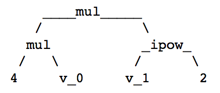
Fig. 10 The binary expression tree of 4*x*y^2.

Then we add the tree N01 to N2345.

N012345 = LabelledBinaryTree([N01, N2345], label='add')
ascii_art(N012345)

We then see the expression tree for x^3 + 4*x*y^2 in Fig. 11.

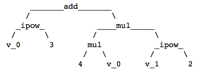
Fig. 11 The binary expression tree of x^3 + 4*x*y^2.

In the next step, we subtract 7*y, as defined in node N67.

N01234567 = LabelledBinaryTree([N012345,N67], label='sub')
ascii_art(N01234567)

We then see the expression tree for x^3 + 4*x*y^2 - 7*y in Fig. 12.

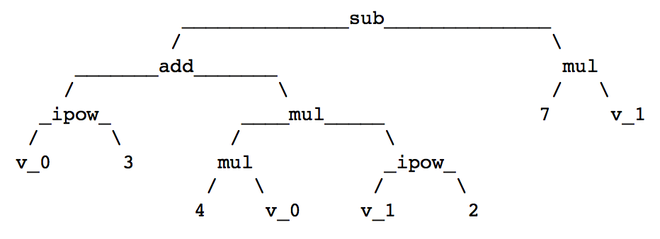
Fig. 12 The binary expression tree of x^3 + 4*x*y^2 - 7*y.

Finally, we add 2 to the tree, where 2 is defined by the last leaf L8.

lbt = LabelledBinaryTree([N01234567, L8], label='add')
ascii_art(lbt)

The final expression tree is shown in Fig. 13.

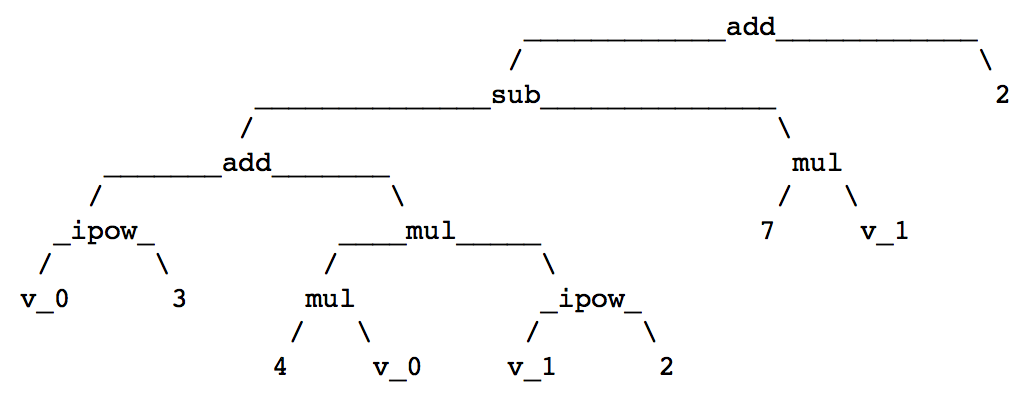
Fig. 13 The binary expression tree of x^3 + 4*x*y^2 - 7*y + 2.

We can obtain a more lower-level representation of expressions:

f = fast_callable(p)
f.op_list()

The output is a list

[('load_arg', 0), ('ipow', 3), ('load_const', 4),
('load_arg', 0), 'mul', ('load_arg', 1), ('ipow', 2),
'mul', 'add', ('load_const', 7), ('load_arg', 1),
'mul', 'sub', ('load_const', 2), 'add', 'return'].

Observe that, if we view the list as a stack, we have a more explicit description to evaluate the expression. We first push the argument of an operand to the stack, the first argument v_0 and then the operator ipow with operand 3. The action of pushing an operator to the stack results in popping the needed operands from the stack, evaluating the operation, and then push the outcome of the operation to the stack, so that this outcome can then be used for the next operation.

Assignments

1. Consider computing modulo 5. This corresponds to computing with numbers in \(Z_5 = \{ 0, 1, 2, 3, 4 \}\). Print the multiplication table for this set of numbers. Explain how you can see from the multiplication table that every element (except for zero) has a multiplicative inverse. Make a loop to print for every nonzero element its multiplicative inverse.

2. Consider polynomials in \(x\) over the modulo 2 integers. List all polynomials of degree at most two and show that \(x^2 + x + 1\) is the only polynomial of degree two or less that does not factor.

3. Let \(p\) be the polynomial \(x^2 y^3 - 3 x^3 + 2 y - 9\). Make a fast callable object for \(p\) and print this object. Use the output of the print of the fast callable object to draw the expression tree to evaluate \(p\).

4. Consider the expression \(2 x^3 y^5 - 6 x^3 + y^8\). Turn this expression into an object of the class ExpressionCall and draw the expression tree with LabelledBinaryTree().