Lecture 7: Number Types and Functions to Store Data
Every object in Sage has a type. The type of an object determines the operations that can be performed on the object. The main data types in Python are lists, dictionaries, and tuples.
The most basic number types in Sage have short abbreviations,
they are ZZ, QQ, RR, and CC, for the integers, rationals,
reals, and complex numbers. We see how to explicitly fix the type of
a number with so-called type coercing.
The ability to choose random numbers is often very useful.
We see how to select left and right hand sides of equations.
The lecture ends with a specific application of default parameters
of functions that enables us to store data in functions.
Coercing to the Basic Number Types
The main number types are integers, rationals, reals, and complex numbers,
respectively denoted by ZZ, QQ, RR, and CC.
To convert from one type to the other is to coerce.
print(ZZ)
We can convert a string in hexadecimal format or octal format into decimal notation.
a = ZZ('0x10'); print(a)
b = ZZ('010'); print(b)
Given the list of coefficients, we can evaluate a number in any base. The following instruction
ZZ(142).digits(10)
returns the list [2, 4, 1] as these are the digits of 142
in the decimal number system , written backwards, starting at
the least significant digit.
Writing 142 in full is \(1 \times 10^2 + 4 \times 10^1 + 2 \times 10^0\).
Passing 3 as the argument of digits(),
we decompose 142 in a number system of base 3, as shown below:
c = ZZ(142).digits(3)
print(c)
print(ZZ(c, base=3))
The last instruction above takes the coefficients
in the list [1, 2, 0, 2, 1] and evaluates the coefficients
as \(1 \times 3^0 + 2 \times 3^1 + 0 \times 3^2 + 2 \times 3^3
+ 1 \times 3^4 = 142\).
A quick way to make a rational representation of a floating-point number
is via type coercing to QQ, the ring of rational numbers.
print(QQ)
x = numerical_approx(pi, digits=20)
y = QQ(x); print(y)
Note the we cannot coerce pi directly to a rational number.
z = RR(y); print(z)
print(QQ(z))
Observe the difference between the value 21053343141/6701487259
of y and the value 245850922/78256779 of QQ(RR(y)).
This is because the precision of RR is the same 53 bit
as the hardware double floats.
print(RR)
print(RDF)
print(RR == RDF)
Although RR has a precision of 53 bits, it is not the same
as the RealDoubleField which is abbreviated as RDF.
Generating random numbers makes the distinction between the
fields RR and RDF a bit more explicit.
The machine precision is the smallest positive number we can add to 1.0 and still make a difference. We can compute the machine precision as follows:
eps = 2.0^(-RR.precision()+1)
print(eps)
Note that the 2.0 in the formula for eps is necessary,
writing 2 instead of 2.0 would have resulted in an exact
rational number, not an element of RR. We see the value
for eps again in the following calculation:
a = 1.0 + eps
a - 1.0
For any real floating-point number x smaller than eps,
the result of 1.0 + x would have remained 1.0.
For any x belonging to some real number field, we can compute
a nearby rational approximation with a given bound on the denominator.
For example x.nearby_rational(max_denominator=1000) returns
a rational approximation for x where the denominator is smaller
than the given bound of 1000.
To compute a sequence of consecutively larger rational approximations,
each time allowing a denominator that is ten times larger than the
previous one in the sequence, we can run the following command.
[x.nearby_rational(max_denominator=10^k) for k in range(1, 11)]
The nearby_rational method gives the third type of rational
approximations for real numbers. The first two we covered were
Rational approximations with prescribed accuracy.
Convergents of the continued fraction representation of the real number.
The application of the method hex() on a real number shows
the hexadecimal expansion of the number.
onetenth = 0.1
onetenth.hex()
The output is 0x1.999999999999ap-4 which does not suggest
a finite expansion. Casting onetenth in a RealField of
a higher precision (e.g.: one hundred bits) will confirm that in binary,
the representation of 0.1 cannot be exact.
Of course, in the decimal notation 0.1
agrees exactly with \(1/10\).
Random Numbers
In simulations, we work with random numbers.
With the method random_element(), we can generate a random
integer number, for example of 3 decimal places, between 100 and 999:
ZZ.random_element(100, 999)
Random real numbers are generated as follows:
x = RR.random_element(); print(x, type(x))
y = RDF.random_element(); print(y, type(y))
The type of x is sage.rings.real_mpfr.RealNumber
while the type of y is sage.rings.real_double.RealDoubleElement.
The same distinction can be made between the Complex Field CC
and the Complex Double Field CDF.
x = CC.random_element(); print(x, type(x))
y = CDF.random_element(); print(y, type(y))
To visualize the distribution of numbers, we can plot a bar chart:
L = [RR.random_element() for _ in range(100)]
bar_chart(L)
Then the output of bar_chart(L) is shown in Fig. 8.
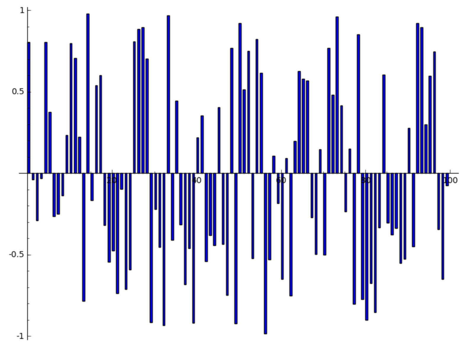
Fig. 8 The bar chart of 100 random numbers.
If we sort the numbers, then we can see that the distribution tends to be uniform.
L.sort()
bar_chart(L)
The sorted numbers are visualized in Fig. 9.
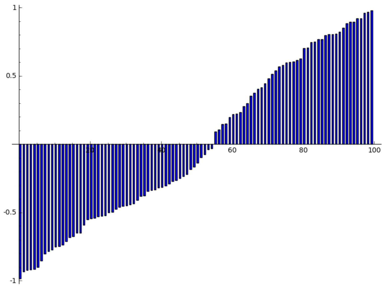
Fig. 9 The bar chart of 100 sorted random numbers.
Components of Expressions
We often work with equations.
eqn = x**2 + 3*x + 2 == 0
print(type(eqn))
The eqn is of type sage.symbolic.expression.Expression,
a type we encountered already many times.
Our expression eqn has an operator.
print(eqn.operator())
The operator is <built-in function eq> and
we can select its left and right hand side
print(eqn.lhs())
print(eqn.rhs())
Alternatives to lhs() are left() and left_hand_side()
and instead of rhs() we may also use right() and right_hand_side().
Storing Data with Functions
The example in this section is taken from the book Sage for Power Users by William Stein.
With default arguments in functions, we can store references to objects implicitly. Consider the following function.
def our_append(item, L=[]):
    L.append(item)
    print(L)
Let us now execute the function a couple times.
our_append(1/3)
our_append('1/3')
our_append(1.0/3)
We see the following lists printed to screen.
[1/3]
[1/3, '1/3']
[1/3, '1/3', 0.333333333333333]
To explain what happened, let us print the address of L each time.
Because we will need to use the address later, we return id(L).
def our_append2(item, L=[]):
    L.append(item)
    print(L, id(L))
    return(id(L))
We run this function our_append2 also three times.
idL = our_append2(1/3)
idL = our_append2('1/3')
idL = our_append2(1.0/3)
and we see the following output
[1/3] 4650781440
[1/3, '1/3'] 4650781440
[1/3, '1/3', 0.333333333333333] 4650781440
The first time we called our_append2 without giving an argument
for the list L, the arguments were evaluated.
The effect of L = [] is that an empty list is created
and placed somewhere in memory.
Each time the function is called with the default
argument of L, the same memory location is used.
Note that the name L does not exist outside the function.
Just to check, print(L) will result in a NameError.
With ctypes we can retrieve the object an address refers to.
idL = our_append2(0)
import ctypes
print(ctypes.cast(idL, ctypes.py_object).value)
Executing the cell shows
[1/3, '1/3', 0.333333333333333, 0] 4650781440
[1/3, '1/3', 0.333333333333333, 0]
Assignments
Try
QQ.random_element(). What do you observe? How would you make a random rational number with type coercions?Type
QQ(pi). Describe what happens. Is this what you would expect? Write a mathematical explanation.Illustrate how you would generate a random complex number of type
CC. The number should have absolute value equal to one. Hint: think about the polar representation of complex numbers.Consider
x = R100(sqrt(2))whereR100is aRealFieldwith a precision corresponding to about 100 decimal places.Compute a list of 10 rational approximations for
x, starting with a 10 as the first bound on the denominator. The bound of the denominator of the rational approximations equals10^kwherekruns from 1 to 10.For each approximation in your list, compute the accuracy, that is the relative error for each rational approximation. Write the relative errors in scientific notation.
Type
eqn = x^3 + 8.0*x - 3 == 0and solve this equation. Verify the solutions in the polynomial defined at the left hand side of the equationeqnwithout retyping the expression at the left hand side of the equation.