Lecture 13: Representation of Expressions

We have already covered expression trees derived from fast callable objects, but a fast callable object is just one representation that is geared for evaluation in hardware arithmetic. In this lecture we examine how expressions in Sage are stored internally.

Expression Trees

Let us consider again the structure of expressions. We generate a random polynomial with rational coefficients.

R.<x,y,z> = PolynomialRing(QQ)
set_random_seed(2018)
p = R.random_element(terms=4, degree=8)
p

Note that we fixed the seed of the random number generator, so we will always see the same polynomial printed.

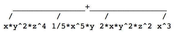
x*y^2*z^4 + 1/5*x^5*y + 2*x*y^2*z^2 + x^3

Unfortunately, the methods operands() and operator() do not work on a multivariate polynomial of this type. We convert p to a general SageMath expression by evaluation in new symbolic variables. Because we will not use the polynomial ring R anymore, we choose the same letters x, y, and z for the new variables.

x, y, z = var('x,y,z')
sq = p(x=x,y=y,z=z)
print(sq, 'has type', type(sq))

Then we see that sq has the same value as p, but is of type sage.symbolic.expression.Expression. We can then ask to see the operands and the operators.

print(sq.operands())
print(sq.operator())

What is printed is [x*y^2*z^4, 1/5*x^5*y, 2*x*y^2*z^2, x^3] and <function add_vararg at 0x1192011b8>. Observe that the list of operands has four elements and that the operator is add_vararg, an addition with a variable number of arguments. Therefore: expression trees of general Sage expressions are NOT binary.

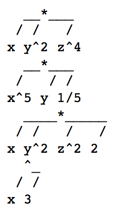
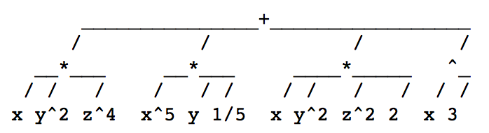
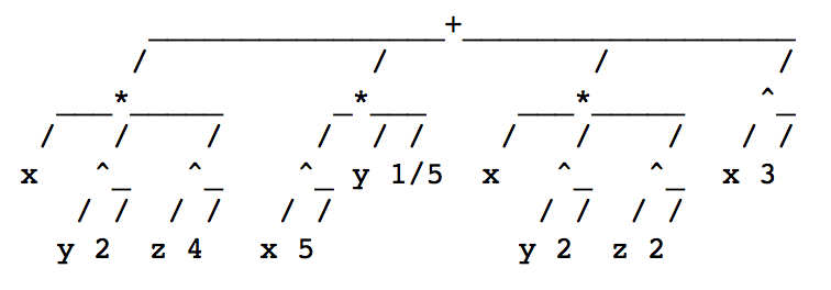
We start drawing the expression tree in a top down fashion.

oplabels = [str(op) for op in sq.operands()]
operands = [LabelledOrderedTree([], label=op) for op in oplabels]
exptree = LabelledOrderedTree(operands, label='+')
ascii_art(exptree)

The top level of the expression tree is shown in Fig. 14.

Fig. 14 The top level of the expression tree of a multivariate polynomial.

We can now apply the same operations to the leaves.

oplabels = [op.operands() for op in sq.operands()]
operands = [op.operator() for op in sq.operands()]
print(oplabels)
print(operands)

All the operators are multiplication, except for the last operator. Because the operands will be used as labels in the new expression tree, we convert to strings.

stroperands = [[str(x) for x in L] for L in oplabels]
print(stroperands)

and we obtain a list of lists:

[['x', 'y^2', 'z^4'], ['x^5', 'y', '1/5'], ['x', 'y^2', 'z^2', '2'], ['x', '3']]

With the list of lists of strings, we make a list of leaves and use the leaves as the internal nodes. The last leaf is dealt with separately.

leaves = [[LabelledOrderedTree([], label=x) for x in op] for op in stroperands]
nodes = [LabelledOrderedTree(leaf, label='*') for leaf in leaves[0:3]]
node3 = LabelledOrderedTree(leaves[3], label='^')
nodes.append(node3)
for node in nodes:
    print(ascii_art(node))

The four nodes are shown in Fig. 15.

Fig. 15 The four nodes at the top level elaborated in the expression tree.

Now we can redefine the expression tree.

exptree = LabelledOrderedTree(nodes, label='+')
ascii_art(exptree)

The redefined expression three is shown in Fig. 16.

Fig. 16 The redefined expression tree with four nodes.

We have five leaves left to elaborate, which are all powers of variables: y^2, z^4, x^5, y^2, z^2.

leafx = LabelledOrderedTree([], label='x')
leafy = LabelledOrderedTree([], label='y')
leafz = LabelledOrderedTree([], label='z')
leafpow2 = LabelledOrderedTree([], label='2')
leafpow4 = LabelledOrderedTree([], label='4')
leafpow5 = LabelledOrderedTree([], label='5')

Now we can define the nodes which represent the powers.

nodeypow2 = LabelledOrderedTree([leafy, leafpow2], label='^')
ascii_art(nodeypow2)

The other nodes are defined similarly.

nodexpow5 = LabelledOrderedTree([leafx, leafpow5], label='^')
nodezpow2 = LabelledOrderedTree([leafz, leafpow2], label='^')
nodezpow4 = LabelledOrderedTree([leafz, leafpow4], label='^')

Apparently there is no way to substitute nodes in a tree. We will manually replace the appropriate entries in the list of leaves and redefine the expression tree.

print(leaves)

The print statement shows

[[x[], y^2[], z^4[]], [x^5[], y[], 1/5[]], [x[], y^2[], z^2[], 2[]], [x[], 3[]]]

Now we redefine the leaves as follows.

newleaves = [[leaves[0][0], nodeypow2, nodezpow4], \
             [nodexpow5, leaves[1][1], leaves[1][2]], \
             [leaves[2][0], nodeypow2, nodezpow2], leaves[3]]
print(newleaves)

and then redefine to obtain the complete expression tree.

nodes = [LabelledOrderedTree(leaf, label='*') for leaf in newleaves[0:3]]
node3 = LabelledOrderedTree(leaves[3], label='^')
nodes.append(node3)
exptree = LabelledOrderedTree(nodes, label='+')
ascii_art(exptree)

The complete expression tree is shown in Fig. 17.

Fig. 17 The complete expression tree of a multivariate polynomial.

Evaluation of Expressions

The form of the expression matters when it comes to evaluation. For fast evaluation, we convert to a fast callable object.

f = fast_callable(sq, vars=['x','y','z'])

Observe the difference in the ways to evaluate:

• with f we do not use the variable names as key words,

• with p we do use the variable names as key words.

print(f(1.0,2.0,3.0))
print(p(x=1.0, y=2.0, z= 3.0))

Both forms of the expression give the same value 397.400000000000. To time the evaluation, we use timeit.

timeit('f(1.0,2.0,3.0)')

We obtain as output 625 loops, best of 3: 11.6 µs per loop.

timeit('p(x=1.0,y=2.0,z=3.0)')

yields 625 loops, best of 3: 92.9 µs per loop. Even already on a such a small example, the fast callable object is much more efficient.

To see the internal structure of the fast callable object f, we apply the method op_list() to it.

f.op_list()

and we see the list of low level instructions which can be interpreted as a stack.

[('load_arg', 0),
 ('load_arg', 1),
 ('ipow', 2),
 'mul',
 ('load_arg', 2),
 ('ipow', 4),
 'mul',
 ('load_arg', 0),
 ('ipow', 5),
 ('load_arg', 1),
 'mul',
 ('load_const', 1/5),
 'mul',
 'add',
 ('load_arg', 0),
 ('load_arg', 1),
 ('ipow', 2),
 'mul',
 ('load_arg', 2),
 ('ipow', 2),
 'mul',
 ('load_const', 2),
 'mul',
 'add',
 ('load_arg', 0),
 ('ipow', 3),
 'add',
 'return']

The data structure which represents a fast callable object corresponds to a binary tree. In a binary tree, every internal node (that is not a leaf) has exactly two children. One reason why fast callable objects are fast is because they are limited to numerical values. The elementary numerical operations such as addition, multiplication, exponentiation are all binary operations and therefore, the expression tree defined by a fast callable object is a binary tree.

Assignments

1. Consider p = 3*x^4 - 6*x^3 + 5*x^2 + 9*x - 7. Draw the expression tree for p. Also give all Sage commands with their output used to make your drawing.

2. Consider p = 3*x^4 - 6*x^3 + 5*x^2 + 9*x - 7. Compute the Horner form q for p and draw the expression tree for q. Also give all Sage commands with their output used to make your drawing.

3. Consider p = 3*x^4 - 6*x^3 + 5*x^2 + 9*x - 7 and its evaluation at math.pi. Compare with timeit the efficiency of the original expression, the Horner q form of p, and the fast callable objects of p and q.

4. Consider the expression:

   \[x + \frac{y}{x^2 - y + 1}.\]

   Draw the internal representation of this expression.