Lecture 24: Symbolic-Numeric Computation

With interval arithmetic we compute floating-point approximations and estimates for the errors. The manipulation of symbolic expressions is used to formulate equations to solve, which we illustrate via the application of the Lagrange multiplier technique to a constrained optimization problem.

Interval arithmetic

There is one important type of arithmetic we have not covered yet, and that is interval arithmetic.

R = RealIntervalField()
R

and R is a Real Interval Field with 53 bits of precision. By default, the RealIntervalField() without argument (also abbreviated as RIF) works with double precision floating-point arithmetic. We can coerce or convert into this field.

api = R(pi)
print(api, 'has type', type(api))
print(api.str(style='brackets'))

and we respectively see 3.141592653589794? (observe the question mark at the end) and the interval [3.1415926535897931 .. 3.1415926535897936] as a RealIntervalFieldElement of sage.rings.real_mpfi.

Interval arithmetic provides operations to add, substract, multiply, and divide intervals. The width of the interval gives an upper bound on the roundoff error. With interval arithmetic we compute at the same time a floating-point approximation and an estimate for the error on this approximation.

To motivate the use of interval arithmetic, we take an example from the paper of Stefano Taschini in the proceedings of SciPy 2008. The problem is to evaluate

\[f(x,y) = (333.75 - x^2) y^6 + x^2 (11 x^2 y^2 - 121 y^4 - 2) + 5.5 y^8 + x/(2y)\]

at \((77617, 33096)\).

To calculate the exact value, we convert the floating-point coefficients to rational numbers.

F(x,y) = (QQ(333.75) - x**2)*y**6 + x**2*(11*x**2*y**2 - 121*y**4 - 2)
+ QQ(5.5)*y**8 + x/(2*y)
print F
(A, B) = (77617, 33096)
exact = F(A, B)
print('the exact value :', exact, RDF(exact))

and the exact value is -54767/66192 or approximated in double precision -0.827396059947. With increasing multiprecision, we may gain more confidence in the results.

f53 = F(A.n(53), B.n(53))
print(f53)
for k in range(54, 105, 10):
    print(F(A.n(k), B.n(k)))

and we see

3.62381792172646e20
-8.18209863729137e20
3.64375473385373696e17
1.46852011835392000000e14
6.72051363840000000000000e10
9.62723840000000000000000000e7
-196610.0000000000000000000000000

Let us continue.

for k in range(100, 130, 5): print(F(A.n(k), B.n(k)))

and then we get the following:

3.9976940000000000000000000000e6
65534.00000000000000000000000000
-2.0000000000000000000000000000000
-2.000000000000000000000000000000000
-2.0000000000000000000000000000000000
-0.7500000000000000000000000000000000000

The sequence of repeated -2.0 values is especially troublesome as one would reach the wrong conclusion that the precision is enough once the sequence has stabilized. This trial and error process is not really encouraging…

R = RealIntervalField(130)
z = F(R(A), R(B))
print(R(z).str(style='brackets'))

and we get

[-0.82812500000000000000000000000000000000000 ..
 -0.82031250000000000000000000000000000000000]

Symbolic-Numeric Factorization

In a numeric factorization of a polynomial in one variable, we compute the complex roots of the polynomial. In a symbolic factorization, we extend the field of rational numbers till the polynomial can be written as a product of linear factors. A symbolic-numeric factorization uses the complex interval field, that is: the roots of the polynomial are computed with complex interval arithmetic in a specific precision. In SageMath, a symbolic-numeric factorization is computed using the QQbar set of numbers.

P.<x> = PolynomialRing(QQbar)

The above statement defines P as the univariate polynomial ring in x over the algebraic field. Any expression in x will be interpreted as belonging to P, as is the case with q below.

q = x^3 + x + 1
factor(q)

We see the three factors of q with the roots written in the interval notation and the I imaginary unit. To see the roots of q over QQbar we can do

q.roots(QQbar)

and we same the same intervals as in the output of factor(q).

If we want a more accurate symbolic-numeric factorization, for example with 200 bits of precision, then we first define a new complex interval field before computing the roots in that new defined field, as done by the code below.

C = ComplexIntervalField(prec=200)
q.roots(C)

Grabbing the output of q.roots(C) defines then the factors in a symbolic-numeric factorization. Computing the product shows the backward error of this computation, that is: the polynomial near to q for which q.roots(C) are the exact roots.

Constrained Optimization

The method of Lagrange multipliers allows to solve a constrained optimization problem.

var('x,y,z')
target = x^2 + 2*x*y*z - z^2
constraint = x^2 + y^2 + z^2 - 1 == 0
print('optimize', target, 'subject to', constraint)

and we get the printed message optimize 2*x*y*z + x^2 - z^2 subject to x^2 + y^2 + z^2 - 1 == 0. To apply the method of Lagrange multipliers, we need to compute the gradients. For this, we convert the expressions into functions. Observe that the constraint was given as an equation, so we must select the left hand side of the equation when we convert the expression to a function.

If we want that the target evaluates at 2, then we see there is no solution, see Fig. 30 made with the commands below.

tplot = implicit_plot3d(target-2, (x,-2,2), (y,-2,2), (z,-2,2), color='red')
cplot = implicit_plot3d(constraint.lhs(), (x,-2,2), (y,-2,2), (z,-2,2))
(tplot+cplot).show()

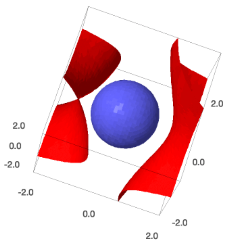
Fig. 30 The blue sphere (constraint) does not touch the red sheets (target at 2).

If we want solutions, then the contraint and target must touch, which is the case when the value of the target equals one. Let us make the plot, see Fig. 31.

tplot = implicit_plot3d(target-1, (x,-2,2), (y,-2,2), (z,-2,2), color='red')
cplot = implicit_plot3d(constraint.lhs(), (x,-2,2), (y,-2,2), (z,-2,2))
(tplot+cplot).show()

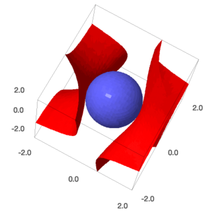
Fig. 31 The blue sphere (constraint) touches the red sheets (target at 1).

ft(x,y,z) = target
fc(x,y,z) = constraint.lhs()
print('target as function :', ft)
print('constraint as function :', fc)
gt = ft.diff()
gc = fc.diff()
print('gradient of target :', gt)
print('gradient of constraint :', gc)

and the results are

target as function : (x, y, z) |--> 2*x*y*z + x^2 - z^2
constraint as function : (x, y, z) |--> x^2 + y^2 + z^2 - 1
gradient of target : (x, y, z) |--> (2*y*z + 2*x, 2*x*z, 2*x*y - 2*z)
gradient of constraint : (x, y, z) |--> (2*x, 2*y, 2*z)

Now we set up the system.

w = var('w')
eqs = [gt(x,y,z)[k] - w*gc(x,y,z)[k] == 0 for k in range(3)]
eqs.append(constraint)
eqs

The polynomial system we obtain is thus

[-2*w*x + 2*y*z + 2*x == 0, -2*w*y + 2*x*z == 0,
2*x*y - 2*w*z - 2*z == 0, x^2 + y^2 + z^2 - 1 == 0]

and then we just do solve…

sols = solve(eqs,[x,y,z,w])
print(sols)
print('found', len(sols), 'solutions')

to see that we found the candidate optimal solutions.

Assignments

1. Do x = RIF(-1, +1); print 1/x. Interpret the result.

2. Compare the evaluation of \(p = x^2 - 4x\) and \(q = x (x-4)\) at the interval [1, 4]. Which form of the expression, \(p\) or \(q\) leads to the most accurate result? Justify your answer.

3. Find those points on the surface \(x^2 - x y + y^2 - z^2 = 1\) closest to the origin. Set up the system with Lagrange multipliers and solve.

4. Consider the surface defined by \(g(x,y) = x^2 + 3 x y + 2 y^2 + 7 x = 0\). Find those points \((x,y)\) that satisfy \(g(x,y) = 0\) and that are closest to the origin.

   1. Define this problem as a polynomial system.

   2. Bring this system in triangular form. How many solutions can this system have? Justify your answer.

   3. Find all real solutions.

5. Consider the function \(f(x) = 1 - 10 x + 0.01 e^x\). Use interval arithmetic to show that \(f(x) = 0\) has a solution in the interval \([9, 10]\).

6. Compute a symbolic-numeric factorization of \(p = x^4 + 3 x^3 + 2 x^2 + x + 9\) with 20 bits of precision. Use the brackets style to display the roots. What is backward error?