Lecture 23: Series, Approximations, and Limits

The manipulation of series is a form of hybrid exact-approximation computation. We start with Taylor series and them move to general power series. The accuracy of Taylor series is only local, for a better global approximation we use Padé approximations, which are rational expressions.

Taylor Series

Let us construct a Taylor series for sin(x) of order 6 at x = 0.

tsin = taylor(sin(x), x, 0, 6)
print(tsin, 'has type', type(tsin))

and we see 1/120*x^5 - 1/6*x^3 + x That the result of taylor is an expression makes it easy for evaluation. Close to zero, this will approximate the true sine function up to 6-th order.

a = tsin(0.01)
b = sin(0.01)
print(a, b, abs(a-b))

which shows the numbers 0.00999983333416667, 0.00999983333416666, and 1.73472347597681e-18 as the magnitude for the error. We can do this pure formally, on an arbitrary function f in x, at some point a.

x, a = var('x, a')
f = function('f')(x)
tf = taylor(f(x), x, a , 4)
print(tf, 'has type', type(tf))

so we get the general form of a Taylor expansion of any function f in x at a as

1/24*(a - x)^4*D[0, 0, 0, 0](f)(a) - 1/6*(a - x)^3*D[0, 0, 0](f)(a)
+ 1/2*(a - x)^2*D[0, 0](f)(a) - (a - x)*D[0](f)(a) + f(a)

The Fibonacci numbers arise as the coefficient of the Taylor series of a particular rational function, called a generating function. To see the first 10 Fibonacci numbers, we can do

g = x/(1-x-x^2)
tg = taylor(g(x), x, 0, 10)
print(tg)
print(tg.coefficients())

The Taylor series is 55*x^10 + 34*x^9 + 21*x^8 + 13*x^7 + 8*x^6 + 5*x^5 + 3*x^4 + 2*x^3 + x^2 + x `` and the coefficients (with corresponding exponents) is are in the list ``[[1, 1], [1, 2], [2, 3], [3, 4], [5, 5], [8, 6], [13, 7], [21, 8], [34, 9], [55, 10]]. Taylor series are defined for expressions in several variables as well. For example, consider cos(x)*sin(y) at x = pi/2 and y = 0.

x, y = var('x, y')
h = cos(x)*sin(y)
taylor(h,(x,pi/2),(y,0),5)

and we get -1/48*(pi - 2*x)^3*y - 1/12*(pi - 2*x)*y^3 + 1/2*(pi - 2*x)*y.

Taylor Series in SymPy

Let us see what systems Sage uses to compute the Taylor series.

from sage.misc.citation import get_systems
get_systems('taylor(sin(x), x, 0, 6)')

and we see ['ginac', 'Maxima'].

Also SymPy exports Taylor series in a more Pythonic way with generators.

from sympy.series import series
series(sin(x), x0=0, n=10)

and the tenth order Taylor series for sin(x) at zero is x - x**3/6 + x**5/120 - x**7/5040 + x**9/362880 + O(x**10). If instead of n=10 for the order, we give None as argument, we obtain a generator:

g = series(sin(x), x0=0, n=None)
print(g, 'has type', type(g))

and we see that g is a generator object. We can use a generator with the next() function to get the next term in the series.

print(next(g))
print(next(g))

or in a list comprehension to get the next 5 terms in the series

[next(g) for k in range(5)]

Power Series

In Sage, Taylor series are not power series, but we can turn any polynomial into a power series.

x = var('x')
q = x^3 + 3*x + 8
pq = q.power_series(QQ)
print(pq, 'has type', type(pq))

and then pq is shown as 8 + 3*x + x^3 + O(x^4) and of type sage.rings.power_series_poly.PowerSeries_poly. Why would we want to turn a polynomial into a power series? Well, unlike polynomials, every power series with a nonzero leading constant coefficient has a multiplicative inverse and there is a division operator for power series.

ipq = 1/pq
print(ipq, 'has type', type(ipq))
print(pq*ipq)

The inverse of the series pq leads to 1/8 - 3/64*x + 9/512*x^2 - 91/4096*x^3 + O(x^4) of the same type as pq. The multiplication leads to 1 + O(x^4). The order of a series is also known as its precision and we can query the precision by the prec() method.

print(pq.prec(), ipq.prec())

So both series are of precision 4. Note that the order is not equal to the degree.

pq.degree()

While the order is 4, the degree is 3.

Truncating to a series of lower precision happens with truncate_powerseries().

tipq = ipq.truncate_powerseries(2)
print(tipq, 'has type', type(tipq))

1/8 - 3/64*x + O(x^2) <type ‘sage.rings.power_series_poly.PowerSeries_poly’> We can turn a power series into a polynomial with the polynomial() method, or we can truncate to a certain precision.

print(ipq.polynomial())
print(ipq.truncate(2))

With polynomial() we see -91/4096*x^3 + 9/512*x^2 - 3/64*x + 1/8 and truncate(2) gives -3/64*x + 1/8.

With r = p.reverse() we compute a power series r so that when r is substituted in p, a series of order k, we obtain x + O(x^k). The series p should not have a nonzero constant term. The coefficients of a series can select with list. Of our example pq, we substract list(pq)[0] to remove the constant term.

print(pq)
print('the coefficients of the series :', list(pq))
pq1 = pq - list(pq)[0]
r = pq1.reverse()
print(r)

What is printed as r is 1/3*x - 1/81*x^3 + O(x^4). Let us verify the reversion of the series by substitution: Note that it works both ways.

pq1(x = r)
r(x = pq1)

and we see x + O(x^4) twice.

Approximations

Padé approximations are rational approximations.

z = PowerSeriesRing(QQ, 'z').gen()
pd = exp(z).pade(4,4)
print(pd, 'has type', type(pd))

and then we see (z^4 + 20*z^3 + 180*z^2 + 840*z + 1680)/(z^4 - 20*z^3 + 180*z^2 - 840*z + 1680). as an object of the class sage.rings.fraction_field_element.FractionFieldElement_1poly_field. How good are the approximations, let us evaluate at 3.14.

print(pd(3.14))
print(exp(3.14))

and we see that we have two decimal places correct:

23.0681517426949
23.1038668587222

Let us compare a power series approximation for \(\sin(x)\) with a Padé approximation.

tsin = taylor(sin(x),x,0,10)
psin = tsin.power_series(QQ)
tsin

The Taylor series of order 10 is \(x - 1/6 x^3 + 1/120 x^5 - 1/5040 x^7 + 1/362880 x^9 + O(x^{10})\). To use as a polynomial we truncate.

polsin = psin.truncate()

The polynomial is not such a good approximation for \(sin(x)\).

sp = plot(sin(x),x,0,2*pi)
pp = plot(polsin(x),x,0,2*pi,color='red')
(sp+pp).show(aspect_ratio=1/4)

The plot is shown in Fig. 28. Observe that after \(x=5\), the Taylor series diverges fast.

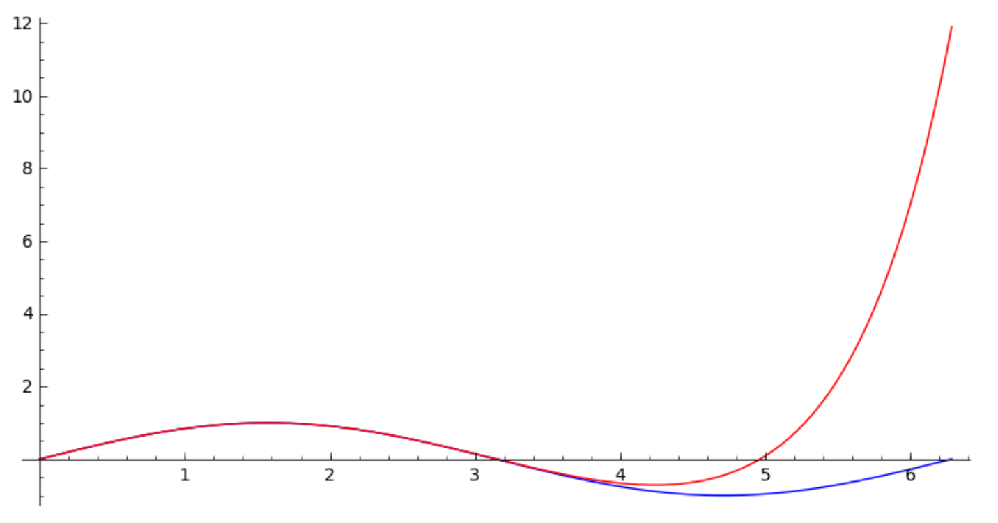
Fig. 28 The plot of the sine function and a 10-th order Taylor approximation.

We can compute a rational approximation for \(sin(x)\), where degree of numerator and denominator are both of degree 7.

z = PowerSeriesRing(QQ, 'z').gen()
pd = sin(z).pade(7,7)
pd

The output is (-479249/18361*z^7 + 7540776/2623*z^5 - 234376560/2623*z^3 + 1644477120/2623*z)/(z^6 + 453960/2623*z^4 + 39702960/2623*z^2 + 1644477120/2623).

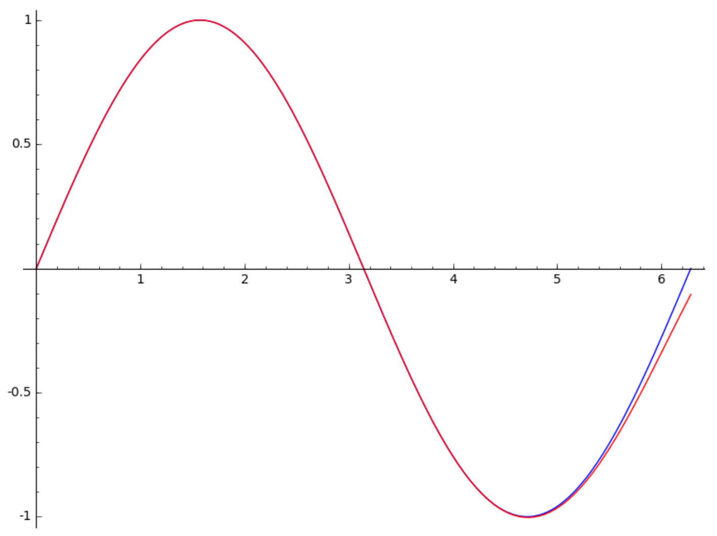
Fig. 29 The plot of the sine function and a 7/7-Padé approximation.

Limits

We can take limits with the limit command. For example, consider the limit definition of the transcendental constant \({\displaystyle e = \lim_{k \rightarrow \infty} \left( 1 + \frac{1}{k} \right)^k}\).

var('k')
f = (1+1/k)^k
f.limit(k=oo)

and as output we see e.

Assignments

1. Make a 10-th order Taylor series of \(\arctan(x)\) about \(x = 0\). Compute the difference between the value of Taylor series evaluated at 0.3 and \(\arctan(0.3)\).

2. Use the series method of SymPy to make a generator for the Taylor series of x/(1-x-x^2) that has the Fibonacci numbers as coefficients. Apply the generator in a list comprehension to compute the first 50 Fibonacci numbers.

3. Use Sage to verify that \({\displaystyle \frac{1}{\sqrt{1 - 4x}} = \sum_{n \geq 0} \left( \begin{array}{c} 2n \\ n \end{array} \right) x^n}\) in the following way:

   1. Compute a 7-th order Taylor series of of \({\displaystyle \frac{1}{\sqrt{1 - 4x}}}\) about \(x = 0\).

   2. Compute \({\displaystyle \sum_{n \geq 0} \left( \begin{array}{c} 2n \\ n \end{array} \right) x^n}\) for \(n = 7\).

4. The binomial coefficient \({\displaystyle \left( \begin{array}{c} n + k \\ k \end{array} \right)}\) counts all choices of \(k\) elements from a set of \(n+k\) elements and can be defined via a Taylor series expansion of \(g(z) = {\displaystyle \frac{1}{(1-z)^{n+1}}}\) at \(z = 0\). Verify this definition for \(n=10\) and all values for \(k\) ranging from 0 to 10.

5. The Catalan numbers arise as the coefficients in the Taylor expansion of the generating function \({\displaystyle \frac{1 - \sqrt{1-4 x}}{2 x}}\).

   Give the Sage command to compute a Taylor series of the generating function at \(x = 0\) of order 10. Compare with the output of catalan_number(10).

6. Compare the accuracy of a Padé approximation for \(\sin(x)\) of (4,4) with the accuracy of a fourth order Taylor series for \(\sin(x)\). Compare with a plot of \(\sin(x)\) on the interval [0, 2].