Lecture 22: Integration and Summation
Integrals occur everywhere in science and engineering. In case there is no symbolic antiderivative, we can approximate the value for a definite integral with numerical techniques.
Indefinite and Definite Integrals
The counterpart to derivative is integral.
integral(cos(x),x)
and we see sin(x).
We can verify that integration is anti-differentiation
and differentiation is anti-integration.
print(diff(integral(cos(x),x),x))
print(integral(diff(cos(x),x),x))
in both cases we see cos(x).
Not every expression has a symbolic antiderivative.
e = cos(exp(x^2))
i = integral(e,x)
print('the anti-derivative of', e, 'is', i)
and Sage prints
the anti-derivative of cos(e^(x^2)) is integrate(cos(e^(x^2)), x)
We can look for the definite integral of the expresion.
d = integral(e, (x, 0, 1))
show(d)
and we see \(\int_{0}^{1} \cos\left(e^{\left(x^{2}\right)}\right)\,{d x}\).
Numerical integration gives an approximation for the definite integral.
d.n()
and we see 0.112823456937.
Assisting the Integrator
We can compute definite integrals symbolically.
var('a, b')
integral(x^2, (x, a, b))
The cubic polynomial -1/3*a^3 + 1/3*b^3 equals the area
under the parabola y = x^2 for all x ranging from a till b.
That does not work always so well.
Sometimes we have to assist the integrator.
var('a, b')
integral(1/x^2, (x, a, b))
The exception triggered is ValueError with the comment that
Computation failed since Maxima requested additional constraints;
and moreover:
using the 'assume' command before evaluation *may* help
(example of legal syntax is 'assume(b-a>0)', see `assume?` for more details)
Before we continue to examine the exception thrown by Sage, let us not see if we cannot apply the fundamental theorem of calculus: (1) compute the antiderivative; and then (2) make the difference of the antiderivatives evaluated at the end points.
ad = integral(1/x^2,x)
print(ad)
print(ad(x=b) - ad(x=a))
The antiderivate is -1/x and evaluated at the end points,
this gives us 1/a - 1/b.
So why does Sage now complain about the original definite integral?
The answer is in the following plot, recall that the definite integral
gives the area under the curve defined by 1/x^2
for all x in [a,b].
Let us take [-1, 1] for the interval.
plot(1/x^2, (x, -1, 1), ymax=100)
The parameter ymax=100 puts a bound on the y-value.
The plot is shown in Fig. 27.
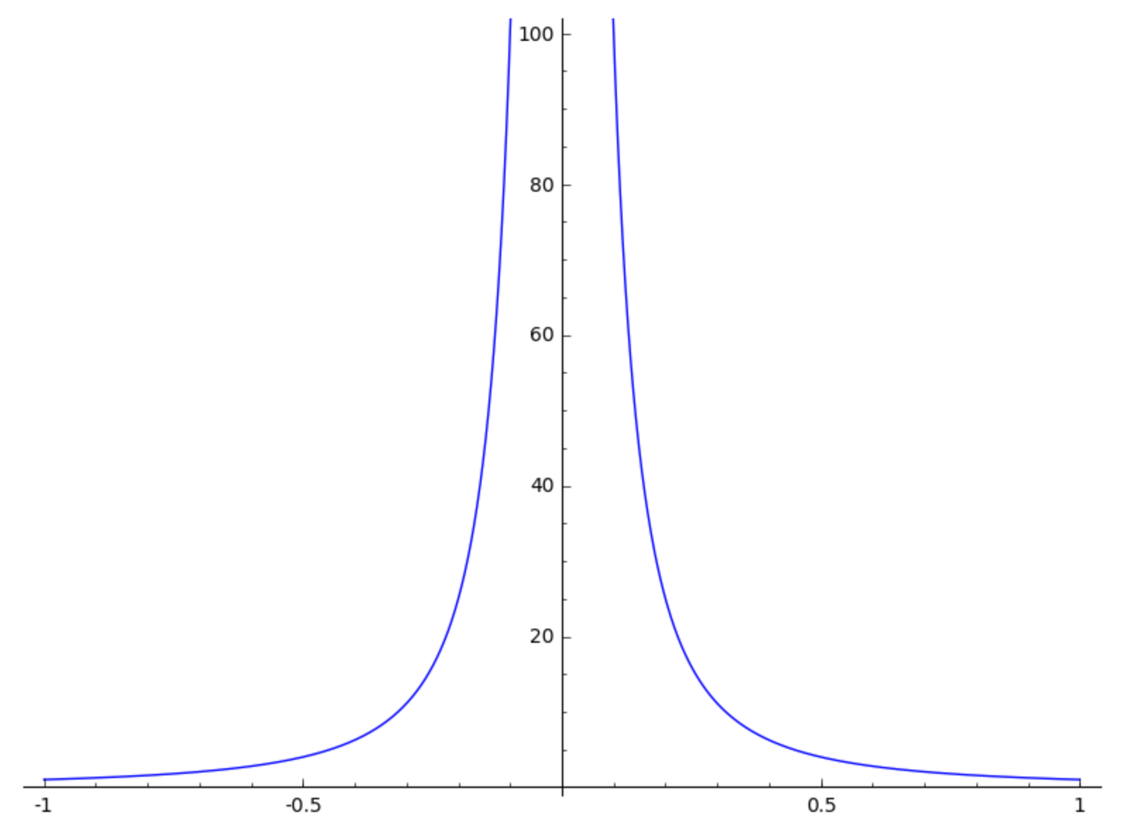
Fig. 27 The function 1/x^2 has an asymptote at x=0.
The plot shows there is something happening in the interval [-1, 1].
Now that we understand that the fundamental theorem of calculus
does not apply for just any interval [a,b], we can look at the
exception Sage raised when we asked for the definite integral.
The question we see in the worksheet is
Is b-a positive, negative or zero?
We see that Sage asks about the sign of b-a. We can add assumptions to variables.
assume(a > 0, b > a)
integral(1/x^2, (x, a, b))
and then we have the value 1/a - 1/b.
We can check the assumptions.
assumptions()
and we then see [a > 0, b > a].
Assumptions are removed with forget.
forget(b > a)
print(assumptions())
forget(a > 0)
print(assumptions())
We then see printed:
[a > 0]
[]
Symbolic Summation
Sage can find explicit expressions for formal sums. Suppose we want to sum k for k going from 1 to n, denoted as \({\displaystyle \sum_{k=1}^n k}\).
var('k, n')
s = sum(k, k, 1, n)
print(s)
f = s.factor()
print(f)
What is printed is 1/2*n^2 + 1/2*n and 1/2*(n + 1)*n
With range and the ordinary Python sum,
we can verify the formulas, say for n = 100.
print(sum(range(1, 101)))
print(f(n = 100))
and in both cases we see 5050 as the sum.
We end with a more interesting formal sum.
Infinity is expressed as oo.
sum(1/k^2, k, 1, oo)
and thus we see that \({\displaystyle \sum_{k=1}^\infty \frac{1}{k^2} = \frac{\pi^2}{6}}\). With list comprehensions, we can verify the symbolic sum with a numerical example.
L = [float(1/k^2) for k in range(1, 100001)]
sqrt(6*sum(L))
and then we see 3.14158310433.
Assignments
Compute \(\int x^n e^x dx\) for a general integer \(n\). Check the result for some randomly chosen values for \(n\).
Let \(F\) be the function defined by \({\displaystyle F(T) = \int_1^T \frac{\exp(-t^2 T)}{t} dt}\).
Define the Sage function \(F\) to compute \(F(T)\). Use it to compute a numerical approximation for \(F(2)\). Compare the approximation for \(F(2)\) to the approximation for \({\displaystyle \int_1^2 \frac{\exp(-2 t^2)}{t} dt}\).
Compute the derivative function of \(F\). What is a numerical approximation of \(F'(2)\)? Compare the value \(F'(2)\) to \(\frac{F(2+h) - F(2)}{h}\) for sufficiently small values of \(h\).
Compute \({\displaystyle \int_0^\infty \frac{\ln(x)}{(x+a)(x-1)} dx}\) for positive \(a\).
Show that \({\displaystyle \sum_{k=1}^n k^3 = \frac{1}{4} n^2 (n+1)^2}\).
Compare the results of \({\displaystyle \int \left( \int \frac{x-y}{(x+y)^3} dx \right) dy}\) with \({\displaystyle \int \left( \int \frac{x-y}{(x+y)^3} dy \right) dx}\). Why are the expressions different?
Compute \({\displaystyle \int_0^1 \left( \int_0^1 \frac{x-y}{(x+y)^3} dx \right) dy}\) with \({\displaystyle \int_0^1 \left( \int_0^1 \frac{x-y}{(x+y)^3} dy \right) dx}\). Is there a correct value for the integral?