Lecture 21: Symbolic and Numeric Differentiation

We can take derivatives symbolically, of expressions and functions. Numerically, we work with difference formulas. Some functions are defined implicitly, as the solution of some equation. Declaring some variables as functions of others, we can derive the equation and solve for the derivative. This is implicit differentiation.

Symbolic Differentiation

We can compute the derivative of an expression with diff, which is an alias for the derivative method.

print('the derivative of cos(x) is', diff(cos(x),x))

and we see that the derivative of cos(x) is -sin(x). For repeated differentiation, we have an extra argument.

[diff(cos(x), x, k) for k in range(5)]

and this list comprehension returns [cos(x), -sin(x), -cos(x), sin(x), cos(x)]. We can compute derivatives of functions.

f(x,y) = x^2*y + 2*x*y + x
print('f =', f)
print('the derivative of f is', f.diff())

The function f = (x, y) |--> x^2*y + 2*x*y + x has as its derivative (x, y) |--> (2*x*y + 2*y + 1, x^2 + 2*x). We see that the derivative of a function in two variables returns a function that returns a tuple of two expressions. This tuple is the gradient of f.

print(f.diff(x))
print(f.diff(y))

and we see the two partial derivatives (x, y) |--> 2*x*y + 2*y + 1 with respect to x and (x, y) |--> x^2 + 2*x with respect to y. What if we take the derivative twice?

f.diff().diff()

we get

[    (x, y) |--> 2*y (x, y) |--> 2*x + 2]
[(x, y) |--> 2*x + 2       (x, y) |--> 0]

The matrix of second order derivatives of a function in several variables is called the Hessian. To compute an element in the matrix we give names of variables as arguments to the diff.

f.diff(x).diff(y)

and we obtain \(\frac{\partial f}{\partial x \partial y}\) as (x, y) |--> 2*x + 2.

Numerical Differentiation

Numerical differentiation is available in scipy.misc, in the derivative method.

from scipy.misc import derivative as numdif
print('exact derivative :', -sin(1.0))
print('1st order approx :', numdif(func=cos, x0=1.0, dx=1.0e-2))

and we then see

exact derivative : -0.841470984807897
1st order approx : -0.841456960361603

The numerical differentiation uses central differences. With extrapolation we can improve the accuracy.

ND = [numdif(func=cos, x0=1.0, dx=1.0e-2, order=k) for k in range(3, 12, 2)]
for a in ND: print(a)
print(-sin(1.0))

what is printed is below

-0.841456960361603
-0.841470984527404
-0.841470984807883
-0.841470984807891
-0.841470984807884
-0.841470984807897

Implicit Differentiation

We can declare derivatives symbolically. Assume one variable y is a function of another variable x.

x = var('x')
y = function('y')(x)
dy = y.diff(x)
print(dy, 'has type', type(dy))

Then dy is a symbolic expression, shown as diff(y(x),x). We need this formal declaration of a function in implicit differentiation.

circle = x^2 + y^2 - 1 == 0
print(circle, 'has type', type(circle))

That y is a function of x shows in the display of the equation x^2 + y(x)^2 - 1 == 0. This equation defines how y depends on x. Then we differentiate the equation.

dc = circle.diff(x)
dc

The equation we now can solve for dy is

2*y(x)*diff(y(x),x) + 2*x == 0

Thus we solve for the derivative.

yx = solve(dc, dy)
yx

The solution is

[
diff(y(x),x) == -x/y(x)
]

The right hand side is the formula for the slope of the tangent line at a point on the circle, as shown in Fig. 26.

Plotting the Tangent Line

Let us make the plot shown in Fig. 26.

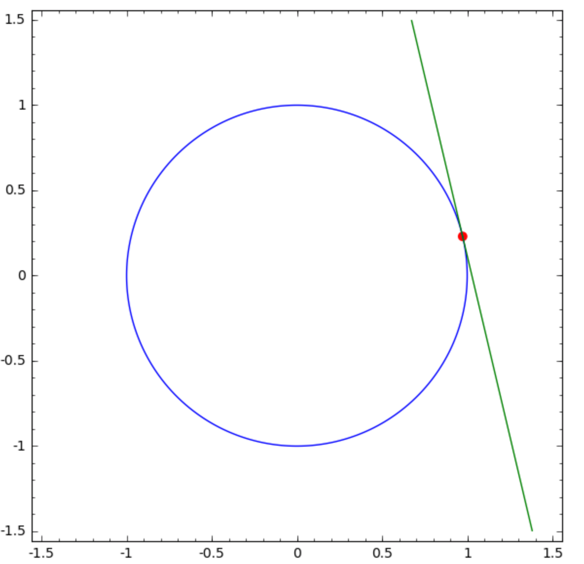
Fig. 26 The tangent line to a point on a circle.

We start by selecting a random point on the circle, randomly chosen in the first positive quadrant. Applying the polar representation of the unit circle, as \((x = \cos(\theta), y = \sin(\theta))\) for some angle \(\theta\), we generate a random number in the interval \([0, \pi/2]\).

angle = RR.random_element(0, pi/2)
circlepoint = (cos(angle), sin(angle))

To compute the slope of the tangent line, we first select the formula for the slope, from the list yx computed above.

slopeformula = yx[0].rhs()

The formula for the slope is -x/y(x) and we will evaluate this formula at the coordinates of the point on the circle, with coordinates in circlepoint. We must apply sequential substitution, first replacing y(x) by the value of the y-coordinate of the point, and then replacing x. A simultaneous substitution will leave the symbol y as a symbol.

slope = slopeformula.subs({y(x):circlepoint[1]}).subs(x=circlepoint[0])

To formulate the equation of the tangent line, we introduce the new variable Y because y is already defined.

Y = var('Y')
tangentline = Y - circlepoint[1] - slope*(x-circlepoint[0])

Then the plotting instructions which yield Fig. 26 are below.

tangent = implicit_plot(tangentline, (x,-1.5,1.5), (Y,-1.5,1.5), color='green')
circle = implicit_plot(x^2+Y^2 - 1, (x,-1.5,1.5), (Y,-1.5,1.5))
plotpoint = point((circlepoint[0], circlepoint[1]), size=50, color='red')
show(circle+tangent+plotpoint)

Assignments

1. Give the SageMath command to compute \({\displaystyle \frac{\partial^8 f}{\partial^5 x \partial^3 y}}\) for \(f(x,y) = e^{2x + \cos(y)}\).

2. Consider the curve defined by the equation 3 + 2 x + y + 2 x^2 + 2 x y + 3 y^2 = 0. Locally we can view y as a function of x, that is: y = y(x). Compute formulas for the first and the second derivative of y with respect to x.

3. Consider the curve defined by the equation \(x^3 - y^2 + x = 0\). The point \(P\) with coordinates \({\displaystyle \left(\frac{1}{2}, \frac{\sqrt{10}}{4}\right)}\) satisfies the equation and thus lies on the curve. Compute the first and second derivatives of the curve evaluated at \(P\). Give the values and the SageMath commands.

4. Consider the plane curve defined by \(p(x,y) = x^4 y^2 - x^2 y^3 + x - y = 0\). Locally at the point \((1,1)\), we view \(y\) as a function of \(x\), that is: as \(y(x)\).

   Compute \(\displaystyle \frac{d y}{d x}\). What is the value for \(\displaystyle y'(1) = \left. \frac{d y}{d x} \right|_{x = 1}\)?

5. Consider the cissoid of Diocles as defined by \(x^3 - (2 - x) y^2 = 0\). What is the slope of the tangent line at \((1,1)\)?