Lecture 20: Computing with Functions

List comprehensions in Python take the form [f(x) for x in L] where L is some list and f some function. The result is a new list that contains all function values of f(x) for all elements x in the list L. In SageMath we can apply list comprehensions to build expressions of arbitrary size and shape.

List Comprehensions

We can use a list comprehension to create a sequence of 20 variables, starting from x01, x02, .., x20.

v = [var('x' + '%02d' % k) for k in range(1,21)]
v

Observe the string concatenation with the proper formatting of the integer index. This leads to the list [x01, x02, x03, x04, x05, x06, x07, x08, x09, x10, x11, x12, x13, x14, x15, x16, x17, x18, x19, x20]. Now we raise every variable to the power three.

p = [x^3 for x in v]
p

and we computed [x01^3, x02^3, x03^3, x04^3, x05^3, x06^3, x07^3, x08^3, x09^3, x10^3, x11^3, x12^3, x13^3, x14^3, x15^3, x16^3, x17^3, x18^3, x19^3, x20^3]. We add up the powers into a sum to make an expression.

e = sum(p)
print(e, 'has type', type(e))

The sum leads to the expression x01^3 + x02^3 + x03^3 + x04^3 + x05^3 + x06^3 + x07^3 + x08^3 + x09^3 + x10^3 + x11^3 + x12^3 + x13^3 + x14^3 + x15^3 + x16^3 + x17^3 + x18^3 + x19^3 + x20^3. We can return to the list representation via the operands() method.

ope = e.operands()
print(ope, 'has type', type(ope))

and this gives a list [x01^3, x02^3, x03^3, x04^3, x05^3, x06^3, x07^3, x08^3, x09^3, x10^3, x11^3, x12^3, x13^3, x14^3, x15^3, x16^3, x17^3, x18^3, x19^3, x20^3]. Raising the k-th operand to the power k goes as follows.

r = [ope[k]^k for k in range(len(ope))]
r

and then we see [1, x02^3, x03^6, x04^9, x05^12, x06^15, x07^18, x08^21, x09^24, x10^27, x11^30, x12^33, x13^36, x14^39, x15^42, x16^45, x17^48, x18^51, x19^54, x20^57]. Note that all operands are expressions.

print(r[2], 'has type', type(r[2]))
print('its degree in' , v[2], ':', r[2].degree(v[2])

With the proper selection of the variable in the argument of degree() we get the right degree, which is 6 for r[2]. We can compute the degrees in their variables.

[(r[k]).degree(v[k]) for k in range(len(ope))]

which leads to [0, 3, 6, 9, 12, 15, 18, 21, 24, 27, 30, 33, 36, 39, 42, 45, 48, 51, 54, 57].

Suppose we want to select those operands of degree less than 13. Recall the unit_step() function.

print(r[2], ':', unit_step(13 - r[2].degree(v[2])))
print(r[8], ':', unit_step(13 - r[8].degree(v[8])))

and we see x03^6 : 1 and x09^24 : 0. Now we can remove all operands with degree higher than 13.

filter = lambda x, k: x*unit_step(13 - x.degree(v[k]))
s = [filter(r[k],k) for k in range(len(r))]
s

and we see [1, x02^3, x03^6, x04^9, x05^12, 0, 0, 0, 0, 0, 0, 0, 0, 0, 0, 0, 0, 0, 0, 0] and then build the expression again with sum().

t = sum(s)
t

and we obtain x05^12 + x04^9 + x03^6 + x02^3 + 1.

Composing Functions

Consider the trajectory of a projectile in space modeled by a parabola, subject to the following constraints. At time t = 0 it is launched from the ground and at time t = 45 it hits the ground 120 miles further. Assuming constant horizontal speed we create a function f(t) to give the altitude of the projectile in function of time. First we model the shape of the trajectory.

y(x) = x*(120 - x)
plot(y(x), (x, 0, 120), aspect_ratio=1/100, thickness=3, color='red')

The parameters thickness and color embellish the plot, adjusting the default value for the aspect_ratio to 1/100 alters the display of the shape of the trajectory, so we do not have to worry about units. The plot is displayed in Fig. 24.

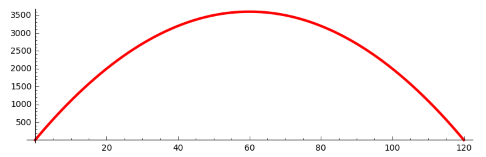
Fig. 24 A parabolic trajectory.

Now we want a function in time t. The assumption of constant horizontal speed implies that x is just a rescaling of t. This means that when t = 45, x must be 120.

x(t) = 120/45*t
print('x at 0 :', x(0))
print('x at 45 :', x(45))

and indeed, we see x at 0 : 0 and x at 45 : 120 printed. Then the altitude is given as the composition of y after x.

f(t) = y(x(t))
print('altitude at 0 :', f(0))
print('altitude at 22.5 :', f(22.5))
print('altitude at 45 :', f(45))

as altitudes at 0, 22.5, and 45, we respectively see 0, 3600.00000000000 and 0. With the composition of functions we have separated the geometric shape of the trajectory and its evolution in time. Suppose we want to halve the speed.

h(t) = t/2
hf(t) = f(h(t))
print('altitude at 45 :', hf(45))
print('altitude at 90 :', hf(90))

and the prints confirm that the projectile reaches its peak at 45 and falls to the ground at 90.

We can also make a 3d-plot of the space curve.

parametric_plot3d([x(t), 0, f(t)], (t, 0, 45), thickness=5, color='red')

and this shows the following image:

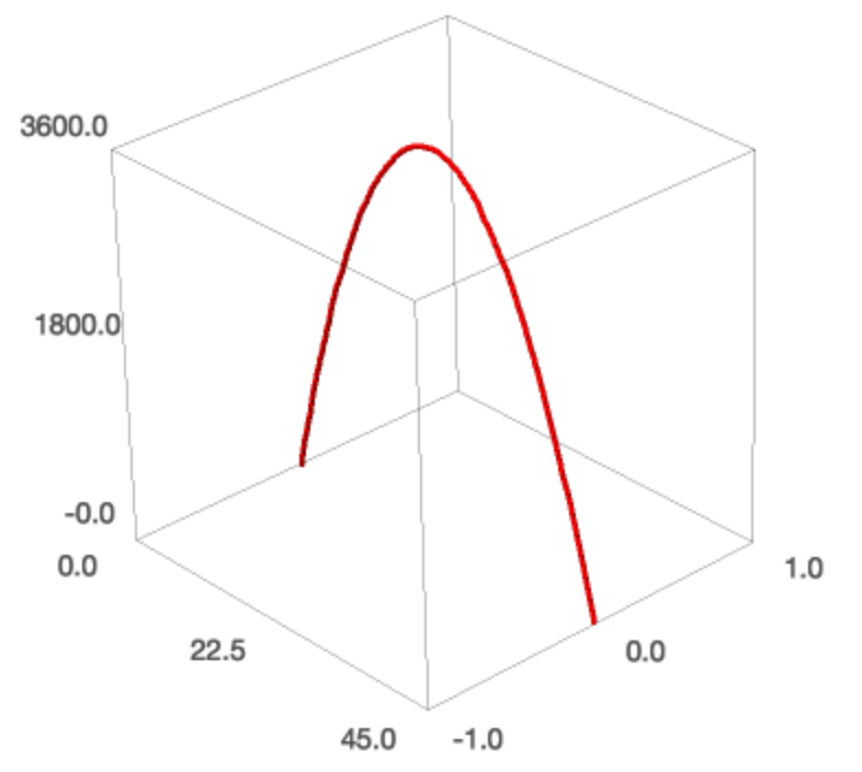
Fig. 25 The parabolic trajectory plotted in three dimensions.

Functions Returning Functions

We can define functions that return functions. Suppose we are interested in solving equations with Newton’s method.

def newton_step(f, x):
    """
    Returns the function that will perform one Newton step
    to solve the equation f(x) = 0.
    """
    n(x) = x - f(x)/diff(f,x)
    return n

Let us try it out on the square function, so we can compute the square root of two.

sqr(x) = x^2 - 2
our_sqrt = newton_step(sqr, x)
our_sqrt

Then we see x |--> x - 1/2*(x^2 - 2)/x. Observe that if we start at an integer value, we get rational approximations for the square root of two.

our_sqrt(our_sqrt(our_sqrt(2)))

Starting at 2, three iterations of Newton’s method yields 577/408. For a repeated application of a function, we multiply strings.

s = 'our_sqrt('*5 + '2' + ')'*5
s

We will then execute our_sqrt(our_sqrt(our_sqrt(our_sqrt(our_sqrt(2))))) and we evaluate the expression.

v = eval(s)
v

This gives 886731088897/627013566048. To compare with an actual approximation for sqrt(2).

print(v.n(digits=30))
print(sqrt(2).n(digits=30))

and we see

1.41421356237309504880168962350
1.41421356237309504880168872421

Assignments

1. Type L = [randint(0,99) for i in range(10)] to generate a list of 10 random numbers between 0 and 99. Give the SageMath commands for the following operations.

   1. divide every element in the list by 100;

   2. convert the list to a list of floating-point numbers of a precision of 3 decimal places;

   3. select all elements in the list that are larger than 0.5;

   4. compute the sum of the elements in the list.

2. The command is_prime() applied to a number returns True if the number is prime and False otherwise. Use is_prime() to make a list of all primes less than 1000. How many 3-digit primes are there?

3. Do P.<x> = PolynomialRing(RR, sparse=False) and then

   q = P.random_element(degree=10).

   Select from q all terms with positive coefficients and make a new polynomial with those terms.

4. For a positive integer \(n\), and a list \(X\) of \(n\) variables \(X\) = [ x1, x2, .. , xn ], define the function

   \[H(n,X,k,c) = 2 n X[k] - c X[k] \left( 1 + \sum_{i=0}^{n-1} \frac{i+1}{i+3} X[i] \right) - 2 n,\]

   where \(c\) is some variable parameter. Show the definition of your function is correct for a list of 9 variables.

5. Let \(n\) and \(k\) be positive natural numbers with \(k < n\) and consider the polynomial \({\displaystyle \sum_{i=0}^{n-1} \prod_{j=0}^{k-1} z_{(i+j) \mbox{ mod } n}}.\)

   Define a function that takes on input a list of variables (where \(n\) is the length of the list) and a value for \(k\). On output is the expression as defined by the polynomial above. Hint: use prod to make the product of a list of expressions.

   Show the result of your function on a sequence of 10 variables and for \(k = 3\).

6. Execute the newton_step function on the our_sqr function, defined again as x^2 - 2. Newton’s method has the property of converging quadratically, that is: in each step the correct number of decimal places doubles. Starting at 2, perform 10 steps with Newton’s method and verify the progess of the accuracy of the rational approximations for the square root of 2? Do you observe quadratic convergence?

7. Define a Python function makeHorner which takes on input the coefficients of a polynomial and the symbol of the variable in the polynomial. For example, if C is [c0, c1, c2, c3, c4] and the variable is x, then makeHorner(C, x) returns

   (((c4*x + c3)*x + c2)*x + c1)*x + c0
   

   Your function makeHorner should directly build the polynomial and not apply the horner() to an expanded polynomial.