Lecture 25: Two Dimensional Plots

Plotting is one of the main strengths of computer algebra systems. We distinguish between plotting formulas and functions. Similar to function and expressions in one variable, curves in the plane are best plotted when given in parametric form. For curves with singularities at the origin, the conversion into a polar form may lead to much better results, because then we can factor out the singular point in the polar formulation.

A plane curve may be given in four different ways. Which command to use depends on the definition of the curve.

1. As the graph of a function \(y = f(x)\): use plot.

2. Implicitly, as an equation \(f(x,y) = 0\), use implicit_plot.

3. In parametric form, as \((x(t), y(t))\): use parametric_plot.

4. In polar coordinates, as \(r = f(t)\): use polar_plot.

Plotting Formulas and Functions

The plot command is for expressions or functions in one variable, that is: we want to see all points \((x,y)\) defined by the function \(y = f(x)\), for all \(x\) in some interval. Note there is a difference in syntax between plotting expressions and functions. We first plot an expression.

x = var('x')
ex = exp(-x^2)*sin(pi*x^3)
plot(ex, x, -2, 2, figsize=4)

The plot produces the plot in Fig. 32.

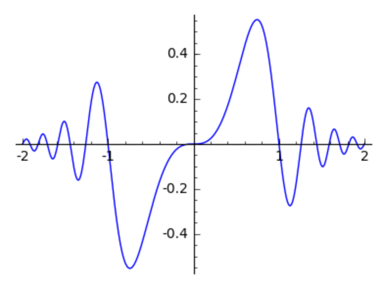
Fig. 32 An example plot of \(\exp(-x^2) \sin(\pi x^3)\).

With a function we do not need to specify the variable name.

ef(x) = ex
plot(ef, -2, 2, figsize=4)

The above plot also shows Fig. 32. We can save plots for later viewing. Another application is to overlay several plots. For the expression above, we will compute the amplitudes separately, as shown in Fig. 33.

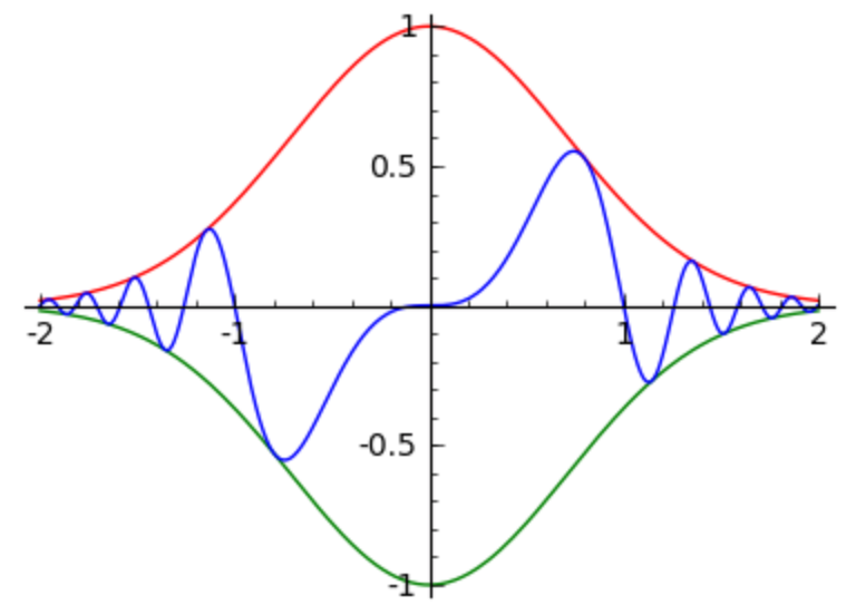
Fig. 33 The curve \(\exp(-x^2) \sin(\pi x^3)\) with amplitudes \(\exp(-x^2)\) and \(-\exp(-x^2)\).

aplus = plot(exp(-x^2), x, -2, 2, color='red')
amin = plot(-exp(-x^2), x, -2, 2, color='green')
explot = plot(ex, x, -2, 2)
graph = aplus + amin + explot
graph.show(figsize=4)

We already use plot on a function with an asymptote (1/x^2, remember?) and that was not pretty, but it did what we wanted to see. For a more pretty picture of a function with an asymptote we can provide extra arguments of plot to limit the viewing window with ymax and ymin.

plot(1/x^2, -2, +2, ymax = 4, figsize=4)

The plot is shown in Fig. 34.

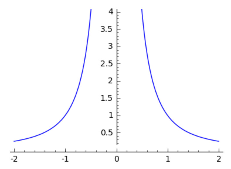
Fig. 34 A plot of an asymptote with a limiting viewing window.

A pole is a root of the denominator, which gives rise to a vertical asymptote. Setting the option detect_poles to True shows no vertical lines. If instead of True we give ‘show’ as value for the option, we see the vertical asymptotes.

plot(1/(x^3 - x),-2,2,ymin=-5,ymax=5,detect_poles='show',figsize=4)

In Fig. 35 we see the vertical asymptotes in the plot.

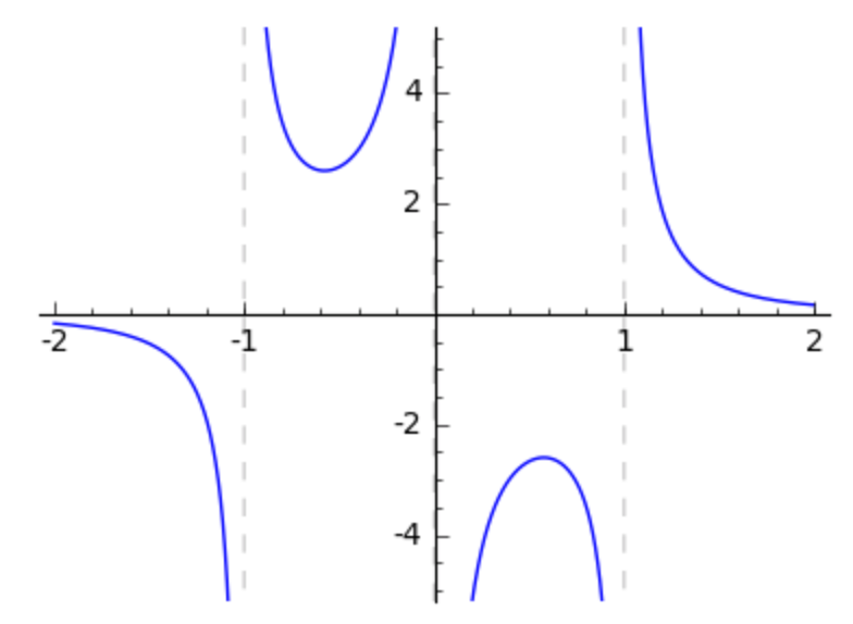
Fig. 35 A plot of a function with multple poles.

Curves in the Plane

Some curves are given by explicit representations for the coordinates \((x(t), y(t))\), as functions in some variable \(t\). We plot such representations via parametric_plot. The Lissajous curve is defined in a parametric way, shown in Fig. 36.

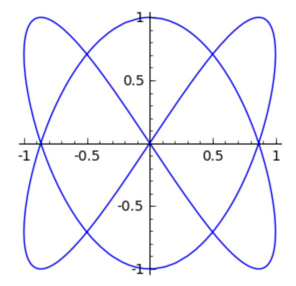
Fig. 36 A plot of a Lissajous curve.

The plot command is below.

t = var('t')
parametric_plot((sin(2*t), sin(3*t)), (t, 0, 2*pi), figsize=4)

Some curves may be given implicitly, via an equation \(f(x,y) = 0\). For the implicit forms, we use the implicit_plot. The curve below is “invented” by James Watt, first shown in Fig. 37 and Fig. 38.

Fig. 37 An implicit plot of \(f = (x^2+y^2)^3 + 5.12 (x^2+y^2)^2 - 5.15(x^4-y^4) - 14.7456y^2\).

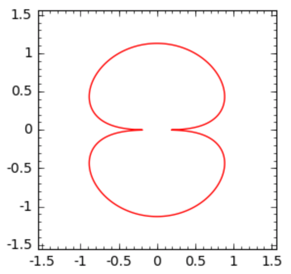
Fig. 38 Another implicit plot of \(f = (x^2+y^2)^3 + 5.12 (x^2+y^2)^2 - 5.15(x^4-y^4) - 14.7456y^2\), using 2000 plotting points.

x, y = var('x, y')
f = (x^2+y^2)^3 + 5.12*(x^2+y^2)^2 - 5.15*(x^4-y^4) - 14.7456*y^2
implicit_plot(f, (x, -2, 2), (y, -2, 2)).show(figsize=4)
implicit_plot(f, (x, -2, 2), (y, -2, 2), plot_points = 2000, \
    color='red').show(figsize=4)

Although the plot made with 2000 points looks very good, we might get the impression that the curve passes twice through the origin.

We will convert to polar coordinates. With polar coordinates, every point is represented by a radius and an angle. The radius is the distance of the point to the origin. The angle is the angle the vector ending at the point makes with the horizontal axis.

r, t = var('r, t')
g = f.subs({x: r*cos(t), y:r*sin(t)})
g

Before solving this expression for r, it is good to simplify.

sg = g.trig_simplify()
sg

Even without factoring we see that r = 0 is a double root.

s = solve(sg,r)

We select the first solution and plot the two parts in different colors. For curves given in polar coordinates, as \(r = f(t)\), we use polar_plot, providing a range for \(t\).

s0 = s[0].rhs()
first = polar_plot(s0, (t, 0, pi), axes=False, color='red')
second = polar_plot(s0, (t, pi, 2*pi), axes=False, color='green')
(first+second).show(figsize=4)

The polar plot is shown in Fig. 39.

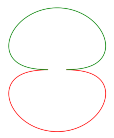
Fig. 39 The two halves of the polar plot, for \(t \in [0, \pi]\) and for \(t \in [\pi, 2 \pi]\).

Is that all? Well, did we not forget the r = 0 component? The point (0, 0) is an isolated singularity of the real curve.

p0 = point((0, 0), color='blue', size=50)
(p0+first+second).show()

The complete polar plot is shown in Fig. 40.

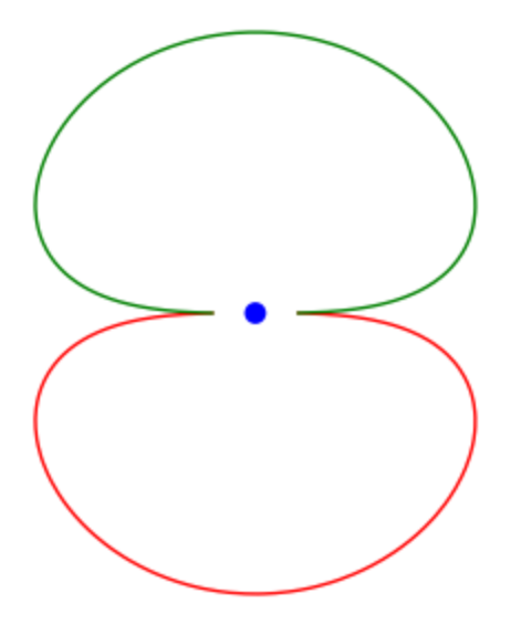
Fig. 40 The complete polar plot with the origin added as a point.

Assignments

1. The neoid is defined by \(r = a t + b\) in polar coordinates. Make a plot for \(a = 0.2\) and \(b = 0.5\), for \(t = 0 \ldots 6\pi\).

2. Consider the curve defined by \(f(x,y) = 4 x y^2 + 2 x^3 - x^2 = 0\) and use SageMath

   1. to convert the equation \(f(x,y) = 0\) from rectangular into polar coordinates;

   2. to solve the equation obtained in (a) for the radius;

   3. to make the plot using the solution(s) obtained in (b).

3. The folium of Descartes is defined by \(x^3 + y^3 = 3 x y\) and has tangent \(x + y + 1 = 0\).

   1. Draw the folium in rectangular coordinates with enough points in the plot, high enough to see a nice smooth curve around the origin. Take \([-2, +2]\) as the range for both \(x\) and \(y\).

   2. Make a plot for the tangent \(x + y + 1 = 0\), using a color different from the plot of the folium. Display both plots on the same figure window. You may want to extend the original range \([-2, +2]\) to see the folium better approaching the tangent.

   3. Convert the folium into polar coordinates and plot. Be careful in choosing a good range for the parameter \(t\). Compare the number of plot points you needed in (a) with the number of plot points that are needed in the polar form.

4. The snail of Pascal is the curve defined as \((x^2 + y^2 + 2 y)^2 - (x^2 + y^2) = 0\).

   1. Plot this curve for \(x \in [-2,+2]\) and \(y \in [-3,+1]\). How many points do you need for the plotted curve to have no gaps?

   2. Compute the polar coordinates for the curve. Plot this curve in polar coordinates.

5. Cassini ovals are sets of points for which the product of the distances to two fixed points are constant. Taking the points on the x-axis with coordinates \((-a, 0)\) and \((+a, 0)\), then for a constant \(c\), the Cassini ovals satisfy \(((x-a)^2 + y^2) \times ((x+a)^2 + y^2) = c^4\).

   1. Make several plots for various choices for \(a\) and \(c\). Distinguish the cases \(0 < a < c\) and \(c < a < c^2\).

   2. Find the representation of these curves in polar coordinates.

   3. Concerning the quality of the plots, is it easier for SageMath to work with the original rectangular coordinates or are the polar coordinates better suited?

6. Consider the curve defined by the equation \(f(x,y) = (x^2+y^2)^5-16 x^2 y^2 (x^2-y^2)^2 = 0\).

   1. Give the command to make a plot of this curve, for \(x\) and \(y\) in the range from \(-1\) to \(+1\). How many points do you need to obtain a good plot?

   2. Give the commands to transform this curve into polar coordinates and to plot the curve. How many times does the curve pass through (0,0)?