Lecture 31: Polyhedral and Unconstrained Optimization

Constrained optimization with Lagrange multipliers was covered at the end of the calculus chapter. Polyhedral optimization asks for the optimal value of a linear function, subject to constraints defined by linear inequalities. The simplex method solves polyhedral optimization problems defined in normal forms. When solving unconstrained optimization problems, the best we can hope to compute are local optima.

Polyhedra

A convex combination of two points is the line segment that has the two points as its ends. Given a set of points, the convex hull of the point is the set of all convex combinations of the points. For points in the plane, this convex hull is a polygon. We can draw a polygon by giving the vertices (or corner points).

Every polyhedron can be defined in two ways:

1. As the convex hull of a list of points.

2. As the intersection of half planes.

The V-representation of a polyhedron P are the vertices that span P (excluding points in the interior). The H-representation of a polyhedron P are the linear inequalities that define the half planes of the intersection that cuts out P.

Let us verify this on 10 random points with integer coordinates between 10 and 99.

set_random_seed(20220722)
xvals = [ZZ.random_element(x=10, y=99) for _ in range(10)]
yvals = [ZZ.random_element(x=10, y=99) for _ in range(10)]
pts = [[x, y] for (x, y) in zip(xvals, yvals)]

The pts contains the list of the points that span the polygon. A polyhedron in the plane spanned by finitely many points is called a polygon.

P = Polyhedron(vertices = pts)
P.plot()

The polygon is shown in Fig. 72.

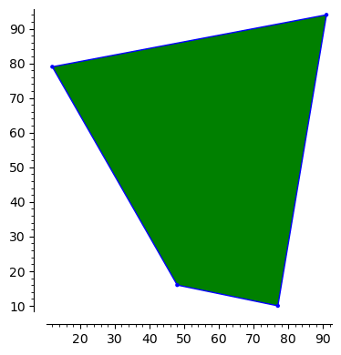
Fig. 72 A polygon generated by ten random integer points.

P.Vrepresentation()

The V-representation of P consists of four vertices, as we can see from the four corners in Fig. 72.

P.Hrepresentation()

The H-representation of P consists of four linear inequalities, as we can see from the four edges in Fig. 72.

Linear Programming

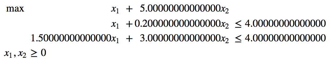
Linear programming optimizes linear functions subject to linear constraints. The following example of a linear program is taken from the Sage documentation.

\[\begin{split}\begin{array}{l} \max x + 5 y \\ \mbox{subject to} \\ \left\{ \begin{array}{lcl} x + 0.2 y & \leq & 4 \\ 1.5 x + 3 y & \leq & 4 \end{array} \right. \end{array}\end{split}\]

where the variables \(x\) and \(y\) are both real and positive. In Sage this can be solved as follows:

p = MixedIntegerLinearProgram(maximization=True)
x = p.new_variable(nonnegative=True)
p.set_objective(x[1] + 5*x[2])
p.add_constraint(x[1] + 0.2*x[2], max=4)
p.add_constraint(1.5*x[1] + 3*x[2], max=4)
p.solve()

and we see 6.666666666666666 as the solution. This solution is the value of the objective at the coordinates of the solution.

The coordinates of the solution can be obtained as follows.

p.get_values(x)

and we obtain the dictionary {1: 0.0, 2: 1.3333333333333333}, implying that with 0.0 as the value for x[1] and 1.3333333333333333 as the value for x[2] the objective attains the optimal value 6.666666666666666.

Let us look at this problem a bit in greater detail.

A = ([1, 0.2], [1.5, 3])
b = (4, 4)
c = (1, 5)
P = InteractiveLPProblem(A, b, c, ["x1", "x2"], problem_type="max", \
              constraint_type="<=", variable_type=">=")
P.plot()

This linear programmig problem is shown in Fig. 73.

Fig. 73 A linear programming problem with the function to optimize drawn in black.

We first convert the problem to its standard form.

P = P.standard_form()
show(P)

The standard form is shown in Fig. 74.

Fig. 74 The standard form of the LP problem of Fig. 73.

The interactive run of the simplex method shows the succession of dictionaries. Let us start with the initial dictionary.

D = P.initial_dictionary()
show(D)

The initial dictionary is in Fig. 75.

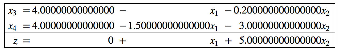
Fig. 75 The initial dictionary to solve the LP problem in Fig. 73.

We ask for the solution, whether the solution is optional, and the value of the objective function.

print(D.basic_solution())
print(D.is_optimal())
print(D.objective_value())

We see (0.000000000000000, 0.000000000000000), False, and 0 as the output of the print statements. The simplex algorithm consists in swapping variables. Variables in the basis are swapped with variables not in the basis. We can ask for the possible variables which can enter the basis.

print(D.basic_variables())
print(D.nonbasic_variables())
etr = D.possible_entering()
etr

The output of the print statements is (x3, x4), (x1, x2), and [x1, x2]. We select the first of the possible entering variables. After setting the entering variable, we ask for the possible variables which can leave the basis.

D.enter(etr[0])
lev = D.possible_leaving()
lev

There is only one possible leaving variable x4. We select the leaving variable and update the dictionary.

D.leave(lev[0])
D.update()
show(D)

The updated dictionary is shown in Fig. 76.

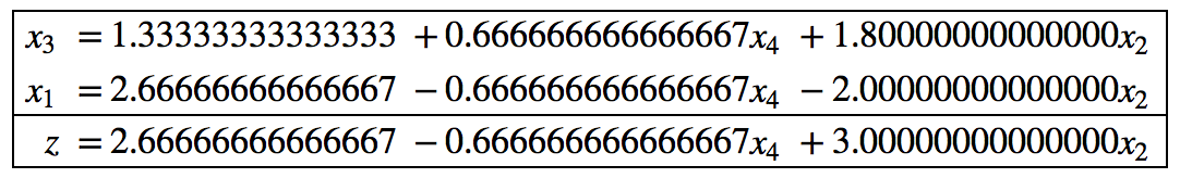
Fig. 76 The updated dictionary after swapping an entering with a leaving variable.

Should we continue? Let us check if the dictionary is optimal and what the objective value is.

print(D.is_optimal())
print(D.objective_value())

We see False and 2.66666666666667 printed, so we have to continue. To continue, let us ask for the possible variables which may enter.

etr = D.possible_entering()
etr

There is only one entering variable x2. After selecting the entering variable, we ask for the possible variables which may leave.

D.enter(etr[0])
lev = D.possible_leaving()
lev

The leaving variable is x1. After selecting the leaving variable, we update the basis.

D.leave(lev[0])
D.update()
show(D)

The updated dictionary is shown in Fig. 77.

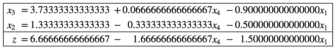
Fig. 77 The updated dictionary after swapping x2 for x1.

Then we check again for optimality.

print(D.is_optimal())
print(D.objective_value())

and we see True and 6.66666666666667 as the objective value.

Unconstrained Minimization

We covered the technique of Lagrange multipliers already to solve a constrained optimization problem. As an example we take a sum of squares.

x, y = var('x,y')
f(x,y) = (3+x-y^2)^2 + (x - 1)^2 + (y - 1)^2
pf = plot3d(f(x,y), (x, -2, 3), (y, -2, 3), adaptive=True, color='automatic',opacity=0.5)
pf.show()

The function f(x,y) defines the surface \(z = f(x,y)\). Minimizing this function has a geometric interpretation. The surface is displayed in Fig. 78.

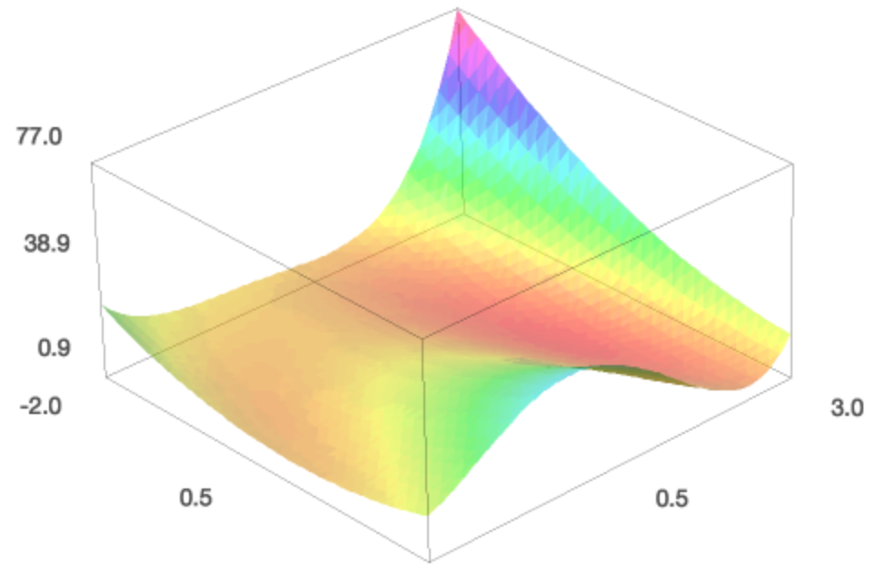
Fig. 78 Looking for the location with the smallest height on a surface.

We can look for a minimum. We need to give an initial guess.

p = minimize(f, x0=[0.0, 0.0], verbose=True)
print('minimum at', p, 'with value', f(p[0], p[1]))

Then Sage prints

Optimization terminated successfully.
         Current function value: 0.882789
         Iterations: 10
         Function evaluations: 14
         Gradient evaluations: 14
minimum at (0.766044177107, 1.87938504258) with value 0.882788808286

To get an idea how good this minimum is we take a look at where the location on the minimum on the surface.

pt = point((p[0], p[1], f(p[0],p[1])), size=20, color='black')
(pt+pf).show()

The point on the surface is shown in Fig. 79.

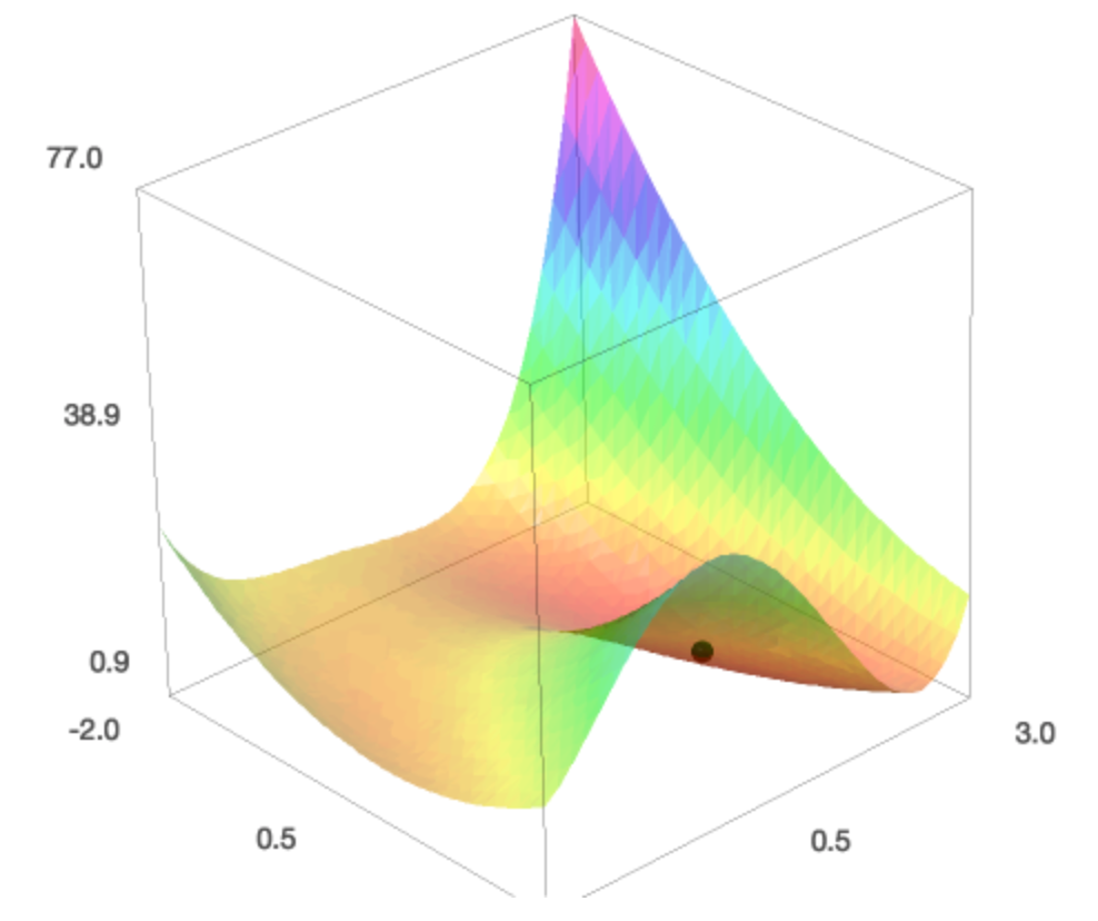
Fig. 79 The computed minimum shown as a black point on the surface.

Assignments

1. Suppose General Motors makes a profit of $100 on each Chevrolet, $200 on each Buick, and $400 on each Cadillac. These cars get 20, 17, and 14 miles a gallon respectively, and it takes respectively 1, 2, and 3 minutes to assemble one Chevrolet, one Buick, and one Cadillac. Assume the company is mandated by the government that the average car has a fuel efficiency of at least 18 miles a gallon. Under these constraints, determine the optimal number of cars, maximizing the profit, which can be assembled in one 8-hour day. Give all Sage commands and the final result.

2. Take the gradient of f(x,y) = (3+x-y^2)^2 + (x - 1)^2 + (y - 1)^2 and solve the polynomial system defined by setting the gradient to zero. The solutions of this system contain the minima of the function. Do you find the outcome of minimize among the solutions of the system?

3. Suppose an invester has a choice between three types of shares. Type A pays 4%, type B pays 6%, and type C pays 9% interest. The investor has $100,000 available to buy shares and wants to maximize the interest, under the following constraints:

   1. no more than $20,000 can be spent on shares of type C;

   2. at least $10,000 of the portfolio should be spent on shares of type A.

   Answer the following questions:

   1. Give the mathematical description of the optimization problem.

   2. Bring the problem into the standard form.

   3. Solve the linear programming problem.

4. Maximize \(2 x_1 + x_2\) subject to \(-x_1 + 2 x_2 \leq 8\), \(4 x_1 - 3 x_2 \leq 9\), \(2 x_1 + x_2 \leq 13\), \(x_1 \geq 0\), and \(x_2 \geq 0\).