Lecture 30: Solving Differential Equations

In Sage, differential equations can be solved with desolve. As the help(desolve) shows, the desolve solves first or second order linear ordinary differential equations via the computer algebra system maxima.

We distinguish between initial value and boundary value problems. The pendulum problem is an example of an initial value problem, the heat diffusion problem is an example of a boundary value problem.

The Pendulum Problem

As our running example of a differential equation, consider a pendulum. We have a mass attached to a string, subject to gravity. The variable is theta(t), the angle of deviation from the vertical position of the string, as a function in time.

t = var('t')
theta = function('theta', t)
theta

In the formulation of the Ordinary Differential Equation (ODE), the gravitational constant is denoted by g, and L is the length of the string. Applying Newton’s laws leads to an equation of second order, involving the second derivative. A more geometrically precise model would have -g*sin(theta), but for small angles theta we simplify sin(theta) to theta.

g, L = var('g, L', domain='positive')

Without declaring g and L as positive the solver will throw an exception. If the domain='positive' is omitted, then one can add the assumptions via assume(g > 0, L > 0).

ode = L*diff(theta,t,2) == -g*theta
ode

The command to solve a differential equation is desolve. We have to tell desolve what is the independent variable, given below in the argument ivar = t.

sol = desolve(ode, theta, ivar=t)
sol

The answer we get is

_K2*cos(sqrt(g)*t/sqrt(L)) + _K1*sin(sqrt(g)*t/sqrt(L))

The _K1 and _K2 in the expression for the solution are general constants. We have two degrees of freedom, as expected for a second order equation. We can formulate an Initial Value Problem. As initial conditions, we assume that we move the mass to an angle of pi/10, with velocity zero. Suppose that at t = 0, we have an initial angle of pi/10, thus: theta(0) = pi/10 and its derivative is 0, so we have D[0](theta)(0) = 0.

sol = desolve(ode, theta, ivar=t, ics=[0, pi/10, 0])
sol

and we see 1/10*pi*cos(sqrt(g)*t/sqrt(L)) as a general symbolic solution to the initial value problem. To plot the solution, we supply values for the gravitational constant g and the length of the string L.

s = sol.subs(g=10, L=3)
print(s)
plot(s, (t, 0, 2*pi))

The plot is shown in Fig. 67.

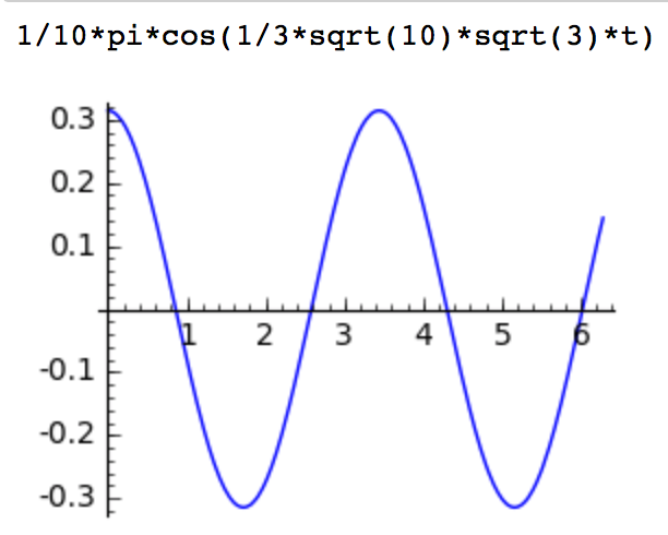
Fig. 67 A specific solution to the pendulum problem.

Plotting the Slope Field

If we solve an initial value problem for particular initial conditions, then we see only one particular solution. With the plot of the slope field we can visualize the whole family of solutions to the problem.

Consider the initial value problem

\[\frac{d y}{d t} = \frac{t^2 + t - y}{t}, \quad y(0) = 1, y'(0) = 3.\]

In formulating the problem, we assign the right hand side of the differential equation in a separate variable rhs because we will need this rhs in the plot of the slope field.

t = var('t')
y = function('y')(t)
rhs = (t^2 + t - y)/t
ode = diff(y,t) == rhs

We solve the ode for y, with initial conditions in ics = [1, 3], expressing that \(y(0) = 1\) and \(y'(0) = 3\).

sol = desolve(ode,y,ics=[1,3])
sol.show()

The solution sol is \(\frac{2 t^3 + 3 t^2 + 13}{6 t}\) and we notice the asymptote at \(t = 0\). Therefore, for a nice plot of the solution, we give lower and upper bounds for the graph in ymin and ymax, restricting the viewing window to \([-50, 50]\). The range for \(t\) is \([-13,13]\).

plotsol = plot(sol,(t,-13,13), ymin=-50, ymax=50, color='red')
plotsol.show()

The plot of the solution is shown in Fig. 68.

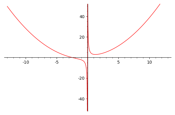
Fig. 68 A plot of a particular solution of an initial value problem.

To plot the slope field we need to take the right hand side of the ordinary differential equation (we saved this on purpose separately in the variable rhs) and replace the y by the solution we found.

plotslopes = plot_slope_field(rhs.subs({y:sol}), \
                              (t, -13, 13), (y, -50, 50), \
                              headlength=4, headaxislength=4, color='green')
plotslopes.show()

With the line breaks separating the arguments of plot_slope_field we indicate the three different types of parameters:

1. the right hand side of the ODE, with substituted y by the solution,

2. the ranges \(t \in [-13,13]\) and \(y \in [-50, 50]\), and

3. the optional arguments for the size and color of the arrows.

The outcome of the above plot_slope_field() command is shown in Fig. 69.

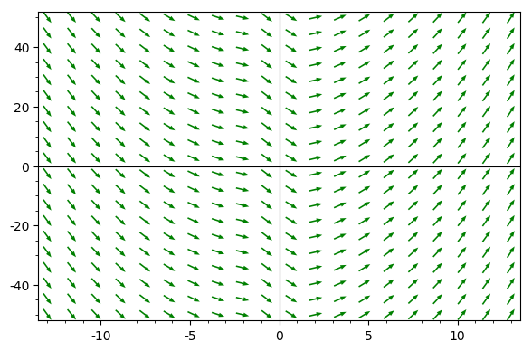
Fig. 69 The slope field of an initial value problem.

To plot both the particular solution and the slope field as shown in Fig. 70, we type (plotsol+plotslopes).show() and

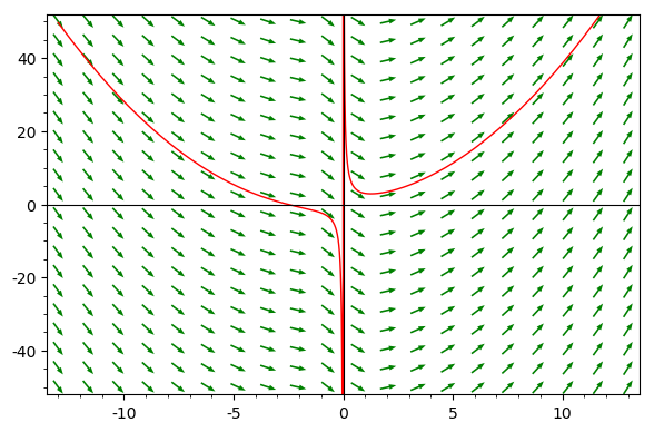
Fig. 70 A particular solution and the slope field of an initial value problem.

Laplace Transforms

One symbolic way to solve differential equations is to use Laplace transforms. Consider a simple model of a swinging pendulum.

t = var('t')
theta = function('theta')(t)
g, L = var('g, L', domain='positive')
ode = L*diff(theta, t, 2) == - g*theta
sol = desolve_laplace(ode, theta, ivar=t)

The solution format has the symbols theta(0) and D[0](theta)(0) for the initial conditions \(\theta(0)\) and \(\theta'(0)\). Storing the initial conditions in a dictionary is convenient for later substitution to obtain a particular solution.

init = {theta(t=0): pi/10, diff(theta,t).subs({t:0}): 0}
sol.subs(init)

which gives 1/10*pi*cos(sqrt(L*g)(t/L) as the solution with parameters L for the length of the string and g for the gravitational constant.

The Laplace transform brings the problem from the time domain into the frequency domain, where the problem can be solved better. We solve the same problem again, but now with the explicit computation of the transform, the solving in the frequency domain, and the application of the inverse Laplace transform. The symbol in the frequency domain is typically s.

s = var('s')
Lode = ode.laplace('t', 's')

The Lode has laplace(theta(t), t, s) as the symbolic representation for the Laplace transform of theta(t). To manipulate this object better, we abbreviate this transform by T via a substitution before solving. Observe that Lode is a linear equation in the Laplace transform.

T = var('T')
Teq = Lode.subs({laplace(theta, t, s): T})
sol = solve(Teq, T)

Selecting the right hand side of the solution, we substitute the initial conditions.

Ts = sol[0].rhs().subs(init)
ft = inverse_laplace(Ts, s, t)

In the last step, the solution was transformed from the frequency domain to the time domain.

Numerically Solving a First Order System

In this section we consider another model of the pendulum, which includes damping. Set \(g/L = 10\) and assume the damping constant to be 1.2. The damping is proportional to the velocity.

\[\frac{d^2}{d~\!t^2} \theta(t) = - 1.2 \frac{d}{d~\!t} \theta(t) - 10 \sin(\theta(t)).\]

To turn this is into a system of first order differential equations, we introduce

\[\frac{d}{d~\!t} \theta(t) = v(t)\]

and obtain

\[\frac{d}{d~\!t} v(t) = - 1.2 v(t) - 10 \sin(\theta(t))\]

Observe that in the last two equations, a first order derivative appears at the left, while on the right only the unknown functions \(\theta(t)\) and \(v(t)\) appear. The format of a system of first order equations is needed for a numerical solver, which will return numerically values.

theta, v = var('theta, v')
rhs = [v, -1.2*v - 10*sin(theta)]
initc = [RR(pi)/10, 0.0]

In addition to the initial conditions, we must provide a range for the time interval.

endtime = 2*RR(pi)
step = 0.1
trange = srange(0, endtime, step)

The numerical solver applies odeint() of SciPy.

sol = desolve_odeint(rhs, initc, trange, [theta, v])

The sol is a matrix of two columns. The first column contains the values for theta, the second column has the values for the velocity v. After selecting the values for theta, we can plot.

angles = sol[:, 0]
pts = [(x, y) for (x, y) in zip(trange, angles)]
p = line(pts)
p.show()

The plot is shown in Fig. 71.

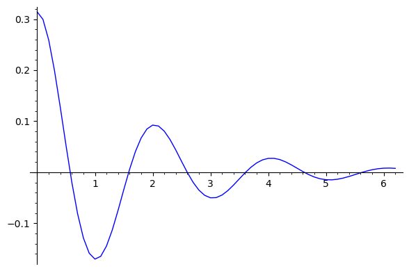
Fig. 71 Trajectory of a pendulum with damping.

Heat Diffusion

As an example of a boundary value problem, consider the diffusion of heat in a rod. We have a rod of length one. The rod experiences temperature differences at its ends. We are interested in the equilibrium temperature distribution, which in its simplest form is expressed as a second order differential equation.

x = var('x')
u = function('u', x)
ode = diff(u, x, 2) == 0
ode

As boundary conditions we impose u(0) = 2.5 and u(1) = 3.1.

sol = desolve(ode,u, ivar=x, ics=[0, 2.5, 1, 3.1])
sol

and we find as solution 3/5*x + 5/2.

Assignments

1. Solve the following initial value problem:

   \[y'' - y = 0, \quad y(0) = 1, \quad y'(0) = 0.\]

   Note that \(y'\) denotes the first derivative and \(y''\) the second derivative with respect to some independent variable.

2. Solve the ordinary differential equation \(3 y^2 y' + 16x = 12xy^2\), where \(y\) is a function of \(x\).

   Describe the form of the computed solution. How can you verify that the expression returned is actually a solution to the equation?

3. Consider the initial value problem which models the motion of a pendulum \(\frac{d \theta}{d t} = -g \theta(t)/L\), for \(g = 10\) and \(L = 3\). The initial values are \(\theta(0) = \pi/10\) and \(\theta'(0) = 0\). Make the plot of the slope field for \(t \in [0, 2\pi]\) and \(\theta \in [-0.4, 0.4]\). Add to this plot the particular solution to this problem.

4. Solve the initial value problem

   \[\frac{d^2 y}{d x^2} + 2 \frac{d y}{d x} + 3 y = \sin(x), \quad y(0) = 1, \quad y'(0) = 0.\]

   Plot the solution for \(x \in [0,20]\) and describe the shape of the solution.

5. Apply Laplace transforms to solve

   \[\frac{d^2}{d~\!t^2} y(t) + y - \sin(2t) = 0,\]

   in the following ways:

   1. Compute first the general solution with desolve_laplace and then substitute the initial values \(y(0) = 2\) and \(y'(0) = 1\) to obtain a particular solution.

   2. Instead of desolve_laplace, compute the Laplace transform of the equation, solve for the Laplace transform \(Y(s)\) of \(y(t)\), followed by the application of the inverse Laplace transform and the same initial values as before.