Lecture 29: Linear Algebra
In this lecture we do linear algebra: we solve linear equations. The formalism to describe linear equations is via matrices. Let us first then look at the matrix types.
Matrices and Linear Systems
With the data in a list of lists, we can make a matrix.
A = Matrix(ZZ,[[1,2],[3,4]])
print(A, 'has type', type(A))
Some matrices are defined by formulas. For example, let us make a 3-by-4 integer matrix where the \((i,j)\)-th entry is \(\frac{1}{i+j}\), for \(i\) and \(j\) both going from 1 to \(n\). Let us make a 3-by-4 matrix with this formula.
B = Matrix(QQ, 3, 4, lambda i,j: 1/((i+1)+(j+1)))
B
Observe that we had to change the formula because in Python as in Sage we count from zero and we do not want 1/0 as the first element in the first row.
We can make a random matrix that way.
C = Matrix(ZZ, 3, 3, lambda i,j: randint(0,10))
C
We can make a random matrix over the rational numbers. In the example below we bound the size of numerator and denominator by 100.
D = random_matrix(QQ, 4, num_bound=100, den_bound=100)
D
A random vector can be made just as easily.
v = random_vector(QQ, 4)
print(v, 'has type', type(v))
We can solve linear systems with the backslash operator (as in MATLAB).
x = D\v
print(x)
print(D*x)
We thus solved with x = A\b the linear system A*x = v.
Matrices over Fields
One way to solve linear systems is via a LU factorization. An LU factorization writes the matrix as a product of a lower with an upper triangular matrix.
A = random_matrix(QQ, 4, num_bound=100, den_bound=100)
print('A =\n', A)
P, L, U = A.LU()
print('L =\n', L)
print('U =\n', U)
print('P =\n', P)
print('P*L*U =\n', P*L*U)
print('A =\n', A)
How does the LU factorization relate to solving linear systems?
Well, because A = P*L*U, the system A*x = b becomes P*L*(U*x) = b,
or if we set y = U*x, then we first solve P*L*y = b and then solve
U*x = y. Let us try if that works on the example, for a random b.
b = random_vector(QQ, 4)
PL = P*L
y = PL\b
x = U\y
print(x)
print(A\b)
We see that x and A\b show the same vector.
Another important decomposition is the eigenvector-eigenvalue decomposition, which for general matrices, diagonalizes the matrix.
A = random_matrix(QQ, 4, 4)
print('A =\n', A)
e = A.eigenvalues()
print('the eigenvalues :\n', e)
We see that the eigenvalues seem numerical:
type(e[0])
but they are of type sage.rings.qqbar.AlgebraicNumber.
The eigenvalues are roots of a polynomial,
the characteristic polynomial of the matrix A.
p = A.charpoly()
print(p)
print(p.roots(QQbar))
print(p.roots(CC))
For an eigenvector z of a matrix with eigenvalue L,
we have A*z = L*z.
Let us verify this property for the first eigenvalue and eigenvector.
The eigenvectors are stored in the columns of the matrix P.
D, P = A.right_eigenmatrix()
Let us verify the relations between the matrices.
print('D =\n', D)
print('the eigenvectors :\n', P)
print('P*D =\n', P*D)
print('A*P =\n', A*P)
We have that A*P = P*D, where D is a diagonal matrix.
Since P is invertible, we have D = P^(-1)*A*P.
p1ap = P.inverse()*A*P
print(p1ap)
print(D)
print(D-p1ap)
The last output is the matrix of very small numbers.
For an eigenvector z of a matrix with eigenvalue L,
we have A*z = L*z.
Let us verify this property for the first eigenvalue and eigenvector.
The eigenvectors are stored in the columns of the matrix P.
v = P[:,0]
print(v)
Av = A*v
Dv = D[0,0]*v
print(Av)
print(Dv)
We see that both vectors Av and Dv are the same.
Matrices over Rings
Recall that in a ring we cannot divide. We can then still solve linear systems with fraction-free row reduction.
The Hermite normal form H of a matrix A is an upper triangular form
obtained by multiplying A with a unimodular transformation U.
A unimodular matrix U has determinant 1 or -1.
A = Matrix(ZZ, 4, 4, lambda i,j: randint(1,10))
print('A =\n', A)
H, U = A.hermite_form(transformation=True)
print('H =\n', H)
print('U =\n', U)
print('U*A =\n', U*A)
We can check the determinants via the det() method.
print('det(A) =', A.det())
print('det(U) =', U.det())
print('det(H) =', H.det())
We see that det(U*A) = det(U)*det(A).
The Hermite normal form is a triangular matrix.
The Smith normal form is a diagonal matrix.
In addition to the diagonal matrix D, the smith_form()
method returns two unimodular matrices U and V.
D, U, V = A.smith_form()
print('D =\n', D)
print('U =\n', U)
print('V =\n', V)
print('U*A*V =\n', U*A*V)
Resultants
With a lexicographic Groebner basis we can eliminate variables and obtain a triangular form of the system. An alternative construction is to use resultants, which are available via Singular. We use Singular when we declare a polynomial ring.
PR.<x,y> = PolynomialRing(QQ)
print(PR)
p = x^2 + y^2 - 5
q = 9*x^2 + y^2 - 9
print(type(p), 'has type', type(q))
We see that PR is then a
Multivariate Polynomial Ring in x, y over Rational Field
and both p and q are of type
MPolynomial_libsingular.
Now we can eliminate one of the variables, say x.
We eliminate from p the variable x with respect to q,
or equivalently, we eliminate from q the variable x
with respect to p.
print(p.resultant(q,x))
print(q.resultant(p,x))
We see the same polynomial 64*y^4 - 576*y^2 + 1296 twice.
Similarly, we can eliminate y
via p.resultant(q,y) and q.resultant(p,y).
With the resultant we can thus compute the coordinates of the roots.
Resultants are determinants of the so-called Sylvester matrix.
sp = p.sylvester_matrix(q, x)
print(sp)
print(sp.det())
The output of sp.det() corresponds to p.resultant(q, y).
Plotting Matrices
We can visualize large sparse matrices via a plot. As an example, we will generate a random matrix of bits.
dim = 32
rm = Matrix(dim, dim, [GF(2).random_element() for k in range(dim*dim)])
rm.str()
For dimensions larger than 32, even plotting with the string method will not give a good view of the pattern of the matrix, whereas a matrix plot scales much better.
matrix_plot(rm, figsize=4)
The plot is shown in Fig. 66.
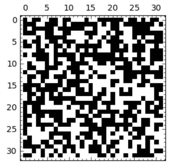
Fig. 66 The plot of a random 32-by-32 matrix.
Assignments
The \((i,j)\)-th entry in an n-by-n Vandermonde matrix is defined as \(x_i^{j-1}\), for i and j both ranging from 1 to n. Give the Sage command(s) to make a 4-by-4 Vandermonde matrix.
Compute the determinant of a 4-by-4 Vandermonde matrix (see the previous exercise). Show that it factors as the product of all differences \((x_i - x_j)\) for \(j > i\) and all i from 1 to 4.
Given a polynomial p in one variable, the companion matrix of p as eigenvalues the roots of p. We will verify this property on a random polynomial.
Generate a monic random polynomial p of degree five. A monic polynomial has its leading coefficient equal to one. Use the Sage command
companion_matrix(look up the help page on its use) to generate the companion matrix of p.Compute the eigenvalues of the companion matrix and compare the eigenvalues with the output of
p.roots(CC).
The \((i,j)\)-th entry of an \(n\)-by-\(n\) Lehmer matrix is \(\displaystyle \frac{\min(i,j)}{\max(i,j)}\), for \(i\) and \(j\) both ranging from 1 to \(n\).
Generate a 5-by-5 Lehmer matrix and verify that all its eigenvalues are positive.
The \((i,j)\)-th entry of the Pascal matrix is defined by \({\displaystyle \left( \begin{array}{c} i+j-2 \\ j-1 \end{array} \right)}\). Make a sparse 32-by-32 matrix, setting the even entries in the Pascal matrix to zero, and the odd entries to one. The
matrix_plotshould show the Sierpinski gasket.A Hankel matrix of dimension \(n\) has first row \({\tt H}[1]\), \({\tt H}[2]\), \(\ldots\) , \({\tt H}[n]\).
The \(j\)-th element on the \(i\)-th row of the matrix equals \({\tt H}[1 + ((i+j-2) ~{\rm mod}~ n)]\), for \(i\) and \(j\) ranging both from 1 to \(n\). Give the Sage command to define a symbolic Hankel matrix \(H_5\) of dimension 5. How many terms does the determinant of \(H_5\) have?