Lecture 28: Solving Equations

In this lecture we solve equations. We start with solving a polynomial in one variable where the coefficients depend on a parameter. Solving this polynomial symbolically requires the application of solve many times. Our running example of a system of polynomial equations is the Apollonius circle problem. A Groebner basis of an ideal in a polynomial ring with lexicographic term order is a triangular basis.

Polynomials in One Variable

Let us consider a polynomial with a parameter A.

A, x = var('A, x')
equ = A^2*(x^2+x+1)-A*(2*x-3) - x^2-3*x+2
equ

Now we can solve for x and obtain symbolic expressions in A as solutions.

s = solve(equ, x)
s

Consider the solutions:

[
x == -1/2*(A + sqrt(-3*A^2 - 10*A + 17) - 3)/(A - 1),
x == -1/2*(A - sqrt(-3*A^2 - 10*A + 17) - 3)/(A - 1)
]

The solutions were obtained via the quadratic formula. But what if we solved for A?

sA = solve(equ, A)
sA

and we get A == -1 and A == (x^2 + 3*x - 2)/(x^2 + x + 1) as solutions. Could A = -1 be a special parameter?

equ.subs(A=-1)

We see 0 and thus, yes, indeed: A = -1 is a special parameter. We just saw that the equation vanishes when A is set to -1. This means that any value for x is a solution. Could there be other special values for A? What happens when we plug in A = 1 in the equation?

equA1 = equ.subs(A = 1)
equA1

When plug in A = 1 we get -4*x + 6. Recall the factor A - 1 in the general solution we first computed. So for A = 1, the solutions we computed before in s are not valid, but there is still a solution, just one single solution.

solve(equA1, x)

and that solution is x == (3/2). Another way we could have detected the special values for A is via the leading coefficient of x in the equation equ.

q = equ.coefficient(x,2)
q

Collecting the terms in x^2 gives A^2 - 1 So the values that kill the leading coefficient of equ are

solve(q, A)

which of course gives A == -1 and A == 1. But then why does one parameter give such different behaviour for the solution x than the other? Let us look at the linear coefficient of the equation in x.

q1 = equ.coefficient(x,1)
q0 = equ.coefficient(x,0)
print(q1)
print(q0)

and the equations q1 and q0 are respectively A^2 - 2*A - 3 and A^2 + 3*A + 2. Then we solve the expressions and we see that A = -1 is a common solution to both the linear and constant coefficient.

print(solve(q1, A))
print(solve(q0, A))

The solutions of q1 are A == 3 and A == -1, while the solutions of q0 are A == -2 and A == -1.

Count the many times we did solve to solve one polynomial equation with parameters and realize that solving equations with parameters symbolically is a much harder problem than solving a polynomial with a numerical coefficients.

Solving Systems of Polynomial Equations

We turn our attention to systems of polynomial equations and solve the circle problem of Apollonius: Given three circles, find all circles that are tangent to the three given circles. An instance of this problem in shown in Fig. 63. Before we get to this, let us first do some exploratory computations with one circle touching the unit circle.

To derive the equations, consider the unit circle and a random circle inside the unit circle. We first plot the unit circle. Because we will solve the equations, we work with implicit_plot(), rather than with the command circle().

x, y = var('x,y')
u = x^2 + y^2 - 1
p0 = implicit_plot(u, (x, -1, 1), (y, -1, 1))
p0.show()

We consider a random circle inside the unit circle. A random circle inside the unit circle has a random center. For reproducible and predictable results, we set the seed of the random number generator.

set_random_seed(2018)
cx = RR.random_element(0, 0.5)
cy = RR.random_element(0, 0.5)
print(cx, cy)
p1 = point((cx, cy), size=50, color='red')
(p0 + p1).show()

The plot is shown in Fig. 60.

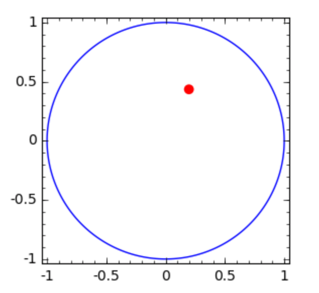
Fig. 60 A random point in the unit circle.

Now the radius of the circle that touches the unit circle is …

r = 1 - sqrt(cx^2 + cy^2)
print(r)
p2 = implicit_plot((x - cx)^2 + (y - cy)^2 - r^2, (x, -1, 1), (y, -1, 1), \
    color='red')
(p0 + p1 + p2).show()

The first circle touching the unit circle from the inside is shown in Fig. 61.

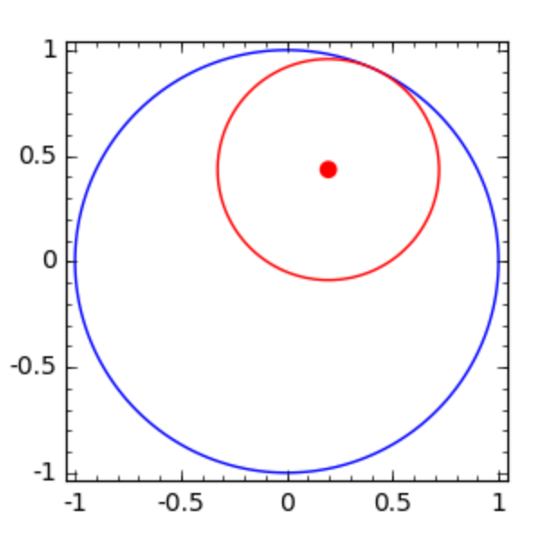
Fig. 61 A circle touching the unit circle from the inside.

We know there is another solution… How to find it?

r2 = 1 + sqrt(cx^2 + cy^2)
p3 = implicit_plot((x - cx)^2 + (y - cy)^2 - r2^2, (x, -2, 2), (y, -2, 2), \
    color='green')
(p0 + p1 + p2 + p3).show()

The other circle which touches the unit circle from the outside is shown in Fig. 62.

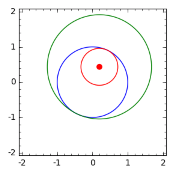
Fig. 62 The second circle touching the unit circle from the outside.

Now we turn our attention to the circle problem of Apollonius. We need three circles on input: The first circle will be the unit circle. The second circle has center (2, 0) with radius 2/3. The third circle has center (1, 1) with radius 1/3.

(c1x, c1y, r1) = (0, 0, 1)
(c2x, c2y, r2) = (2, 0, 2/3)
(c3x, c3y, r3) = (1, 1, 1/3)
c1 = (x-c1x)^2 + (y-c1y)^2 - r1^2
c2 = (x-c2x)^2 + (y-c2y)^2 - r2^2
c3 = (x-c3x)^2 + (y-c3y)^2 - r3^2
xr = (x, -1, 3); yr = (y, -1, 2)
p1 = implicit_plot(c1, xr, yr)
p2 = implicit_plot(c2, xr, yr)
p3 = implicit_plot(c3, xr, yr)
(p1 + p2 + p3).show()

The input to the Apollonius circle problem is shown in Fig. 63.

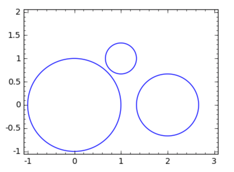
Fig. 63 Find all circles which touch three given circles.

Now we look for the circle that will be tangent to all three circles.

r = var('r')
e1 = (x - c1x)^2 + (y - c1y)^2 - (r - r1)^2
e2 = (x - c2x)^2 + (y - c2y)^2 - (r - r2)^2
e3 = (x - c3x)^2 + (y - c3y)^2 - (r - r3)^2
eqs = [e1, e2, e3]
eqs

and now we solve the system. We set the option solution_dict to True because this works better to select the coordinates of the solution.

sols = solve(eqs, (x, y, r), solution_dict=True)
sols

We see there are two solutions, computed exactly.

s0x = sols[0][x]
s0y = sols[0][y]
s0r = sols[0][r]
print(s0x, s0y, s0r)
sc0 = implicit_plot((x-s0x)^2 + (y-s0y)^2 - s0r^2, (x, -2, 3), (y, -3, 2), \
    color='red')
s1x = sols[1][x]
s1y = sols[1][y]
s1r = sols[1][r]
print s1x, s1y, s1r
sc1 = implicit_plot((x-s1x)^2 + (y-s1y)^2 - s1r^2, (x, -2, 3), (y, -3, 2), \
    color='red')
(p1 + p2 + p3 + sc0 + sc1).show()

The plot of two circles touching three given circles in shown in Fig. 64.

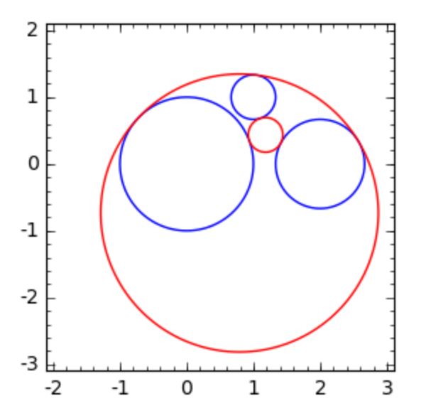
Fig. 64 Two of the eight circles touching three given circles.

Note that this problem has actually 8 solutions in total. What we computed are only types. Instead of (r-r1), we should also consider (r+r1).

Groebner Bases

We saw that the system was solved exactly, via what looked like the quadratic formula. We will cast the polynomial equations in a polynomial ring with lexicographic order.

PR.<x,y,r> = PolynomialRing(QQ, order='lex')
print(PR)
q1 = PR(e1)
print(q1, 'has type', type(q1))

We see that PR is a Multivariate Polynomial Ring in x, y, r over Rational Field and the polynomial q1 has type MPolynomial_libsingular so we will be using the computer algebra system Singular. to work with the polynomials of the Apollonius circle problem. We also cast the other two polynomials into this ring and define the ideal generated by the three polynomials. An ideal generated by polynomials in a ring consists of all combinations of the generators with elements in the ring.

q2 = PR(e2); q3 = PR(e3)
qs = [q1, q2, q3]
J = Ideal(qs)
J

A Groebner basis of an ideal in a polynomial ring with lexicographic term order is a triangular basis.

B = J.groebner_basis()
B

The Groebner basis for the ideal generated by the polynomials of the Apollonius circle problem is

[x + 1/6*r - 41/36, y + 1/2*r - 11/36, r^2 - 71/39*r - 253/468]

We see that the last polynomial is a quadratic polynomial in one variable, that is r. Recall that r was the last variable in our lexicographic term order. The other two polynomials are linear and we can express x and y as functions of r.

We can ask for the solution set defined by the polynomials in the ideal J by asking for its variety:

J.variety()

If we provide no argument to variety() then the default field is QQ and only the rational solutions will be returned. For more general approximations, we provide the extended field QQbar.

J.variety(QQbar)

The returned solutions are approximated by intervals.

Assignments

1. Consider the polynomial equation \(x^2 a^2 - 12 x^2 + a^2 x - 3\sqrt{3} a x + 6 x + a^2 - \sqrt{3} a - 6 = 0\).

   Give the Sage command to solve the equation with \(x\) as variable.

   For which values of the parameter \(a\) does the equation have less than two solutions?

   Find the solution for this special value of the parameter.

   For which values of the parameter \(a\) does the equation have infinitely many solutions?

   Give the Sage commands you used to test your answer.

2. There are eight different solutions to the Apollonius circle problem, which can be obtained by considering instead of r - r1 also r + r1 and likewise for the radii r2 and r3. Make a plot that shows all eight different solutions as shown in Fig. 65.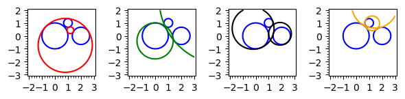

   

   Fig. 65 The four pairs of solutions to the problem of Apollonius.

3. Solve the system

   \[\begin{split}\left\{ \begin{array}{r} x^2 + y^2 - 5 = 0 \\ 9 x^2 + y^2 - 9 = 0 \end{array} \right.\end{split}\]

   Make a plot of the two algebraic curves to confirm the values found for the intersection points.

   How many solutions did you find? How many solutions do you see?

4. As an illustration of the technique of Lagrange multipliers we derived the system in the list below:

   [-2*w*x + 2*y*z + 2*x == 0, -2*w*y + 2*x*z == 0,
   2*x*y - 2*w*z - 2*z == 0, x^2 + y^2 + z^2 - 1 == 0]
   

   Compute a Groebner basis for a ideal generated by the four polynomials in the list above, with a lexicographic term order.

   Explain how you can compute the number of solutions from the triangular structure of the Groebner basis.

5. A comet approaches earth in an ellipsoid path, defined by \((x-2)^2/6 + y^2/2 - 1 = 0\), where the earth is at the center \((0,0)\) of our coordinate system.

   We want to know the locations where the comet is closest to earth.

   1. Set up the polynomial system to find those locations.

   2. Solve the polynomial system and find the coordinates on the ellipse closest to the origin.

   3. Make a plot of the ellipse and the solution found in (b).