Lecture 27: Animations

An animation is defined by a list of plots, which will make the frames of the movie. We will show various examples of animations with the several plotting commands we have covered so far.

As in the previous lecture, our browser is google chrome and we use the Sage Math Cloud.

Animating Plots

Let us start with a two dimensional plot of a sine function with a vanishing amplitude. The plot is shown in Fig. 52.

t = var('t')
f = exp(-t^2)*sin(2*pi*t)
plot(f, (t, -2, 2))

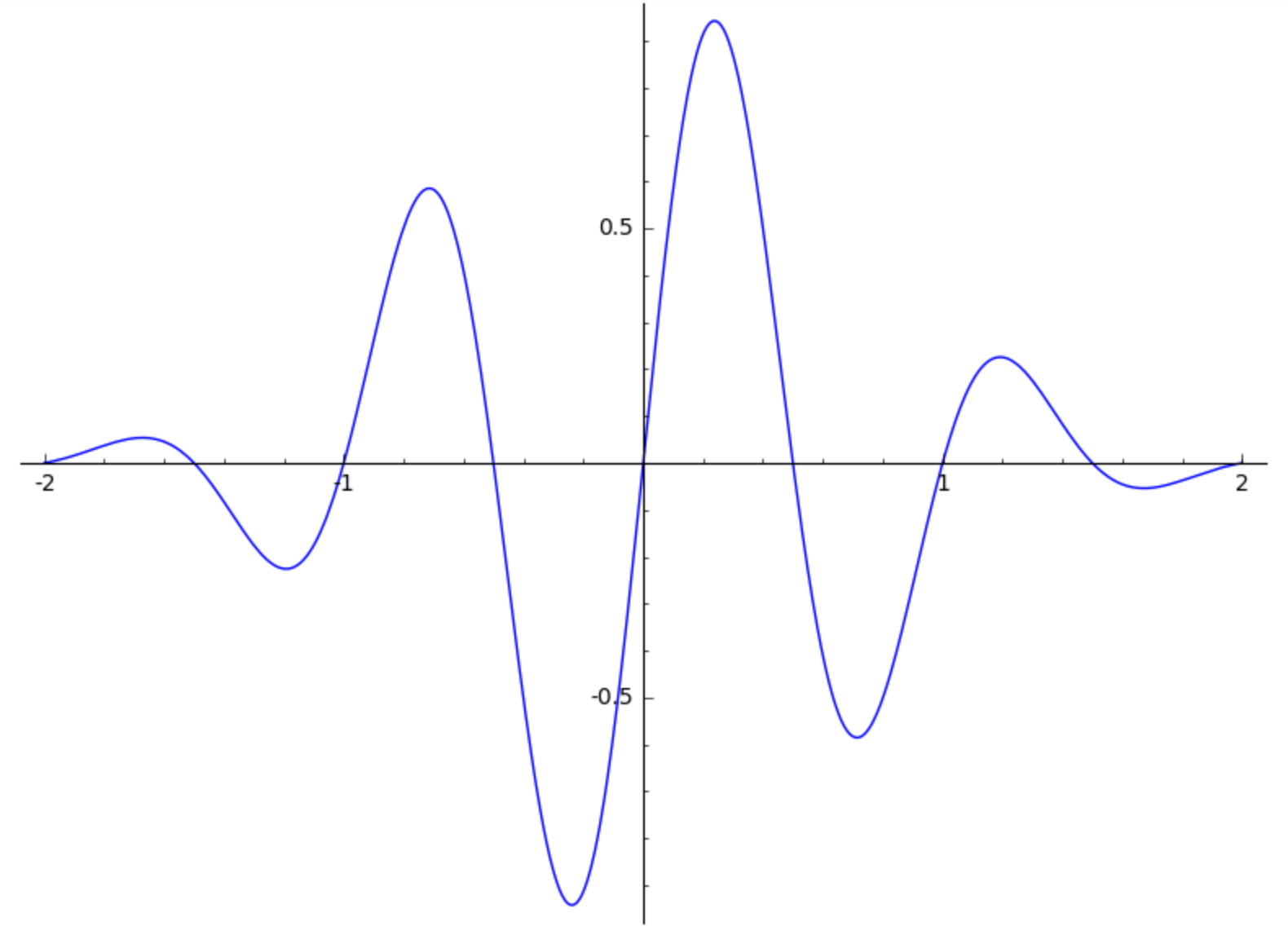
Fig. 52 The first frame in an animation.

The argument of the sine function is set so the frequency equals one, for t going from 0 to 1, the argument of sine goes for 0 to 2*pi. Suppose we want to see the evolution as we increase the frequency from 1 to 10. With a list comprehension, we make a sequence of plots. This list defines the frames in our animation. To test whether we did not make any mistakes in setting up the list of plots, we render the first frame. What we see is the same as in Fig. 52.

frames = [plot(exp(-t^2)*sin(2*k*pi*t), (t, -2, 2)) for k in range(1,11)]
frames[0].show()

And then, we just call the animate command on the list of frames.

animate(frames)

That is it! We can regulate the speed of the animation by providing a value for the parameter delay, for example: animate(frames, delay=10). By default, the animation runs in an infinite loop. Giving a value for the parameter iterations fixes the number of iterations, for example: animate(frames, iterations=4).

An animation can be turned into a graphics_array, suitable for viewing all frames (or selection of the frames) at once. We assign the animate(frames) to a and select the first 5 frames of the animation.

a = animate(frames)
g = a[:5].graphics_array(ncols=5)
show(g,figsize=[8,2], axes=False)

The first five frames of the animation are shown in Fig. 53.

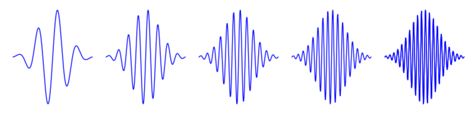
Fig. 53 The first five frames in an animation, via a graphics_array.

We can save an animation as a gif file:

a.save('ouranimation.gif')

The name between quotes may need be extended with the absolute path name if we do not want the animation to be saved in the current folder.

Designing an Animation

Interesting animations consists of several moving parts. Consider the animation of the tangent line to a circle. The ten frames are shown in Fig. 54.

Fig. 54 Ten frames in the animation of the tangent lines to a circle.

For the first frame, we draw the unit circle and the first point at angle \(2 \pi/10\) and coordinates \((\cos(2 \pi/10), \sin(2 \pi/10))\).

unitcircle = circle((0,0),1)
firstpoint = point((cos(2*pi/10), sin(2*pi/10)), color='red',size=50)
(unitcircle+firstpoint).show(figsize=3)

The circle and point for the first frame are shown in Fig. 55.

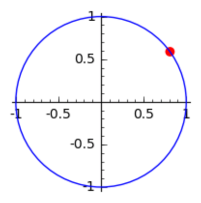
Fig. 55 A point on a circle in the first frame of the animation.

Now we make a list of points. The angle will be \(2 k pi/10\), for \(k\) ranging from 1 to 10. In the arguments of the animate command, we must specify values for the boundaries of the viewing window, for the xmin, xmax, ymin, ymax, because otherwise the point remains fixed and the coordinate axes are moving.

movingpoints = [point((cos(2*k*pi/10), sin(2*k*pi/10)), \
   color='red', size=50) for k in range(1,11)]
a = animate(movingpoints,xmin=-1,xmax=1,ymin=-1,ymax=1)
a.show(iterations=3)

For the tangent line, we know that vectors perpendicular to \((\cos(t), \sin(t))\) are \((-\sin(t),\cos(t))\) and \((\sin(t), -\cos(t))\). These two perpendicular vectors are added to \((\cos(t),\sin(t))\) to compute the end points of the tangent line. We define functions to make the points because we will generate lists of plots to make the frames of the animation.

pt(k) = (cos(2*k*pi/10), sin(2*k*pi/10))
v1(k) = (-sin(2*k*pi/10), cos(2*k*pi/10))
v2(k) = (-v1(k)[0],-v1(k)[1])
A(k) = ((pt(k)[0]+v1(k)[0]),pt(k)[1]+v1(k)[1])
B(k) = ((pt(k)[0]+v2(k)[0]),pt(k)[1]+v2(k)[1])

The function pt defines the coordinates of the moving point. The functions A and B given the end points of the tangent line. Now we are ready to plot the first frame in the animation.

tangentline1 = line([A(1), B(1)],color='green')
(unitcircle+firstpoint+tangentline1).show(figsize=4)

The first frame of the animation is shown in Fig. 56.

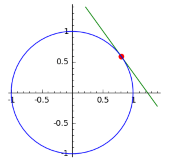
Fig. 56 The tangent to the first point on the circle in the animation.

The extra work to define the functions pays off as the definition of the 10 frames for the moving tangent lines is straightforward. Observe how the plot for the unit circle is added to each plot of a new tangent line.

movinglines = [unitcircle+line([A(k), B(k)], color='green') \
   for k in range(1,11)]
a = animate(movinglines,figsize=4,xmin=-1.5,xmax=1.5,ymin=-1.5,ymax=1.5)
g = a.graphics_array(ncols=10)
g.show(axes=False, figsize=[10,10])

The outcome of the above commands are shown in Fig. 57.

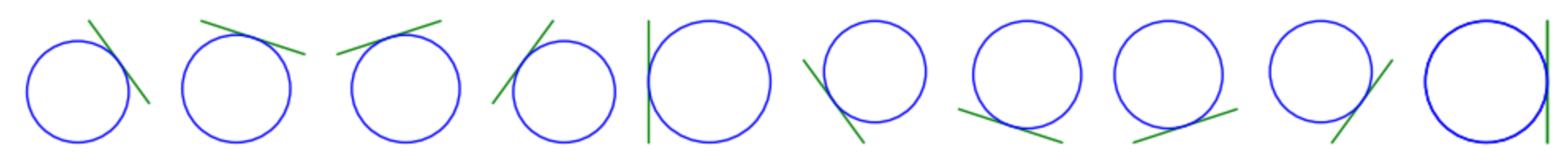
Fig. 57 The ten frames in the plot of tangents to the unit circle.

Then finally, we can make the animation.

frames = [movinglines[k]+movingpoints[k] for k in range(10)]
a = animate(frames, figsize=4, xmin=-1.5, xmax=1.5, ymin=-1.5, ymax=1.5, \
            axes=False)
a.show()

The frames in the animation are shown in Fig. 54.

Animating Surfaces

A first natural animation of a surface is to make a spin plot, for various orientations of the coordinate axes. For example, consider the parabolic cylinder defined by \(x^2 - y = 0\). We let the x-axis rotate, with 20 frames, for the angle \(2 k \pi/10\), for math:k ranging from 1 to 20.

x, y, z = var('x, y, z')
Xframes = [implicit_plot3d(x^2 - y, (x, -1, 1), (y, 0 , 1), \
           (z, -1, 1)).rotateX(k*2*pi/10) for k in range(1, 21)]
Xa = animate(Xframes)
Xa.show()

and the animation shows a rotating parabolic cylinder. Replace the rotateX by rotateY or rotateZ to have the cylinder tumbling in a different direction.

Our next animated surface is a rotating plane. We consider the family \(z = (1-k/20) x + k/20 y\), for \(k\) ranging from 0 to 20.

x, y = var('x,y')
frames = [plot3d((1-k/20)*x + k/20*y, (x,-1,1), (y,-1,1)) \
    for k in range(0, 21)]
animate(frames, xmin=-1, xmax=1, ymin=-1, ymax=1, zmin=-1, zmax=1)

For \(k = 0\) we have \(z = x\) and for \(k = 20\) we have \(z = y\).

Animating Space Curves

A space curve in parameter form is defined by three functions in one parameter, defined over some range. We can visualize the growing of the space curve by letting the parameter range grow, as illustrated by the following knot.

reset()
t = var('t')
r = 2 + 4/5*cos(7*t)
z = sin(7*t)
curve = [r*cos(4*t), r*sin(4*t), z]
parametric_plot3d(curve,(t, 0, 2*pi), thickness=5)

The above plot uses the range (t, 0, 2*pi) for t to range in the entire interval, which closes the knot. To view the growth of the knot, define the frames as follows:

frames = [parametric_plot3d(curve,(t,0,2*k*pi/20), thickness=5) \
          for k in range(1,21)]
a = animate(frames, xmin=-3, xmax=3, ymin=-3, ymax=3, zmin=-3, zmax=3)
a.show()

Observe that the number of plot points remains the same. In a better animation, the number of plot points would increase with each frame.

Assignments

1. Make an animation of ten frames of the plot of \(\exp(-t^2) \sin(2 \pi t)\), for \(t\) starting at \(-2\) and ending at \(-2+2 k/5\), for \(k\) ranging from 1 to 10.

   The frames of the animation are displayed in Fig. 58.

   

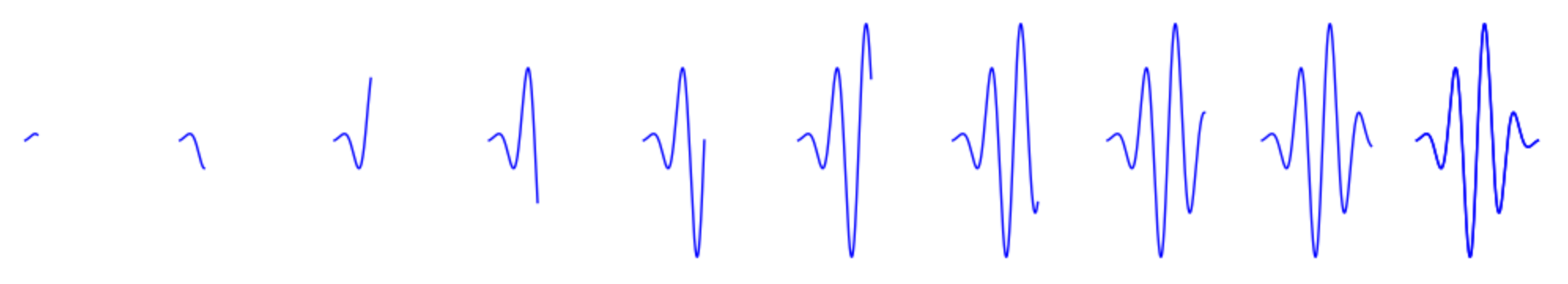
   Fig. 58 An animation of a plot with increasing right bound for the variable.

2. The neoid is defined by \(r = a t + b\) in polar coordinates.

   Give the Sage commands to produce an animation of 10 frames, for \(a = 0.2\) and for \(b\) going from 0.1 to 1, and for \(t = 0 \ldots 6 \pi\).

3. Make an animation of a spiral, using the formulas \(x = t \cos(t)\), \(y = t \sin(t)\), and \(z = t\). Let there be 30 frames in your animation, with \(t = 1,2, \ldots, 30 \pi\).

4. The Viviani curve is a space curve defined by \(x = R \cos^2(t)\), \(y = R \cos(t) \sin(t)\), and \(z = R \sin(t)\), where \(R\) is some parameter.

   Make an animation for the curve for \(R\) going from 1 to 10 (thus using ten frames). Give all Sage commands you use to make this animation.

5. Make an animation to show the drawing of the golden rectangle, using 14 frames shown in Fig. 59.

   

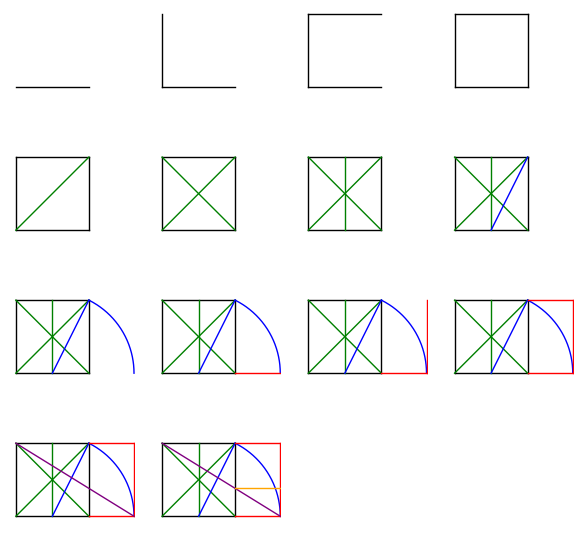
   Fig. 59 Drawing the golden rectangle with ruler and compass.