Lecture 34: Building Interactive Web Pages

We can view an interactive web page as a graphical user interface, with the main difference that we need a browser to run the interaction.

At UIC, the computer people.uic.edu offers web hosting to students, staff and faculty. If Apache runs on your computer, then you can run the web pages by pointing your browser to localhost.

We follow chapter 6 in the book of Gregory Bard and work through the tangent-line interact.

Drawing Tangent Lines to a Curve

The code below is adapted from Sage for Undergraduates by Gregory Bard, pages 285 in Figure 1.

f(x) = x^3 - x
df(x) = diff(f(x), x)
def tangent_at_point(x0):
    """
    Shows the tangent line at the point x0,
    using f and its derivative as global variables.
    """
    y0 = f(x0)
    slope = df(x0)
    # y - y0 = slope*(x - x0) implies
    # y = slope*x - slope*x0 + y0
    b = y0 - slope*x0
    P1 = plot(f, -2, 2, color='blue', ymin=-6, ymax=6, gridlines='minor')
    P2 = plot(slope*x + b, -2, 2, color='tan', ymin=-6, ymax=6)
    P3 = point((x0, y0), color='red', size=50)
    P = P1+P2+P3
    P.show(figsize=3)

To test the script we run the following cases in separate cells.

tangent_at_point(0.5)
tangent_at_point(1.5)
tangent_at_point(-1.75)

The three figures for the x-coordinates 0.5, 1.5, and -1.75 are respectively displayed in Fig. 80, Fig. 81, and Fig. 82.

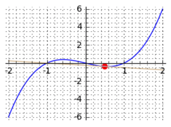
Fig. 80 The tangent line of \(x^3 - x\) for \(x=0.5\).

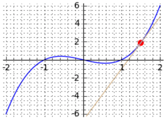
Fig. 81 The tangent line of \(x^3 - x\) for \(x=1.5\).

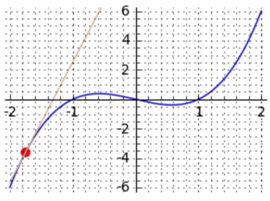
Fig. 82 The tangent line of \(x^3 - x\) for \(x=-1.75\).

We want to attach a scale to the x0 parameter of the function. When the user then moves the scale, the point on the curve will move and the tangent line at that new point will be shown. To the code we add @interact before the function definition. In the header of the function we add the slider.

The parameter x0 of the function is extended into x0 = slider(-2, 2, 0.1, -1.5, label='x-coordinate'). The first two arguments, -2 and 2 determine the range of the slider, so x0 is constrained to take values in the interval with bounds -2 and 2. The granularity of the slider is defined as 0.1, the third parameter of the slider(). The fourth parameter sets the initial value -1.5 of x0.

f(x) = x^3 - x
df(x) = diff(f(x), x)
@interact
def tangent_at_point(x0 = slider(-2, 2, 0.1, -1.5, label='x-coordinate')):
    """
   Shows the tangent line at the point x0,
   using f and its derivative as global variables.
   """
   y0 = f(x0)
   slope = df(x0)
   # y - y0 = slope*(x - x0) implies
   # y = slope*x - slope*x0 + y0
   b = y0 - slope*x0
   P1 = plot(f, -2, 2, color='blue', ymin=-6, ymax=6, gridlines='minor')
   P2 = plot(slope*x + b, -2, 2, color='tan', ymin=-6, ymax=6)
   P3 = point((x0, y0), color='red', size=50)
   P = P1+P2+P3
   P.show()

If we execute the code in the cell, then we can already test the interact as it would run in a web page. The interact is shown in Fig. 83.

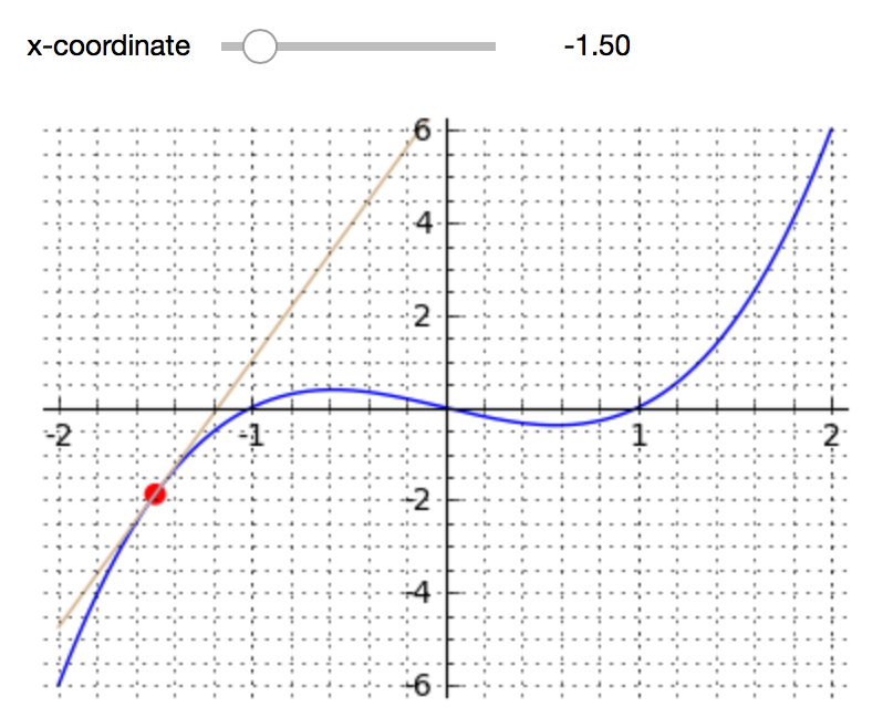
Fig. 83 An interact with a slider to set the x-coordinate of a point.

Making the Web Page

On page 294 of Sage for Undergraduates by Gregory Bard, we have a template of a web page, based on work of Jason Grout. Once we insert the code in the last cell of the previous section, we are ready to publish the interactive web page.

The computer people.uic.edu which can host your web pages is a Linux computer. You can login to this computer with your netid. Your web site is accessible via the URL https://netid.people.uic.edu where the netid in the URL is replaced by your netid. Below is a description of the steps to deploy the interact on your web site.

1. Login to people.uic.edu via ssh, available among the internet tools on the lab computers.

2. The files which defined your web pages should be placed in the folder public_html. Make sure that this folder is accessibile. To make public_html accessible, execute the command chmod +x public_html at the command line.

3. You can edit the html file locally on your computer and then transfer the file into the public_html folder on people.uic.edu with a secure copy which can be found among the internet tools on the lab computers.

Note that you account on people.uic.edu needs to be activated. Point your browser to people.uic.edu to activate.

Drop Down Menu

With selector we add a drop down menu to let the user choose from a range of options. For example, to select a color.

fun = x^3 - x
rng = (x, -2, 2)
@interact
def colorplot(colrgb=selector(['red', 'green', 'blue'], label='color: ')):
    """
    Plots the expression defined by fun over the range in rng.
    The parameters fun and rng must be defined before calling colorplot.
    The user can select the color.
    """
    P = plot(fun, rng, color=colrgb)
    P.show()

The result of the interact is shown in Fig. 84.

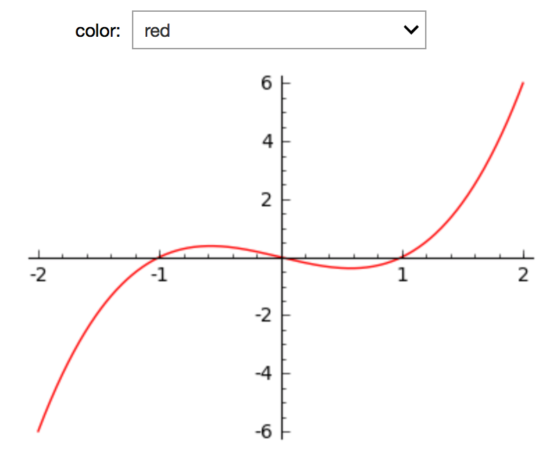
Fig. 84 An interact with a selector to let the user select a color.

Assignments

1. Consider the function \(f(x) = \exp(-x^2) \sin(2 k \pi x)\) for \(x \in [-2,+2]\) and for \(k\) ranging from 1 to 10. Make an interactive web page that plots \(f(x)\) and with a slider so the user can set \(k\).

2. When plotting in three dimensions we can rotate the axes, for example with the rotateX method. Make an interactive plot3d method where the argument for rotateX can be manipulated with a slider.

3. Cassini ovals are all points at distance \(c\) from the points with coordinates \((-a,0)\) and \((a, 0)\), and satisfy

   \[((x-a)^2 + y^2)((x+a)^2 + y^2) = c^4.\]

   Define an interact that plots the Cassini ovals for \(x\) and \(y\) in \([-4,4]\) which lets the user select the parameters \((a,c)\) from the tuples (1,2), (2,1), and (2,3).

4. The coordinates of the Lissajous curve are defined by

   \[x(t) = \sin(2 t), \quad y(t) = \sin(3 t), \quad t \in [0, 2 \pi].\]

   Write the code to define an interact to plot this curve.

   • The interact allows the user to set the end of the range for \(t\) with a slider.

   • The range always starts at 0. The smallest value for the end of the range is \(\pi/20\). The largest value of the end of the range is \(2 \pi\).

   • The end value for the range is incremented by \(\pi/20\).

   • The initial value for the end of the range is \(2 \pi - \pi/10\).