Lecture 35: an Application of Interact
In this lecture we consider an application of interact. We build a model of a four bar mechanism. The mechanism is attributed to Chebyshev and it transmits straight to circular motion. We build the interact in three stages, first the crank, then we solve a polynomial system to determine the coordinates of the connector point. In the third stage we add the coupler point and the fourth bar. Our interact is shown in Fig. 85.
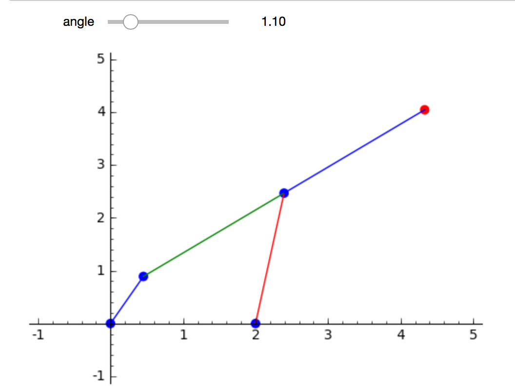
Fig. 85 An interact to draw the Chebyshev 4-bar mechanism.
To learn more about the Chebyshev mechanism, see for example Kinematics, Dynamics, and Design of Machinery by Kenneth J. Waldron and Gary L. Kinzel, second edition, John Wiley & Sons, 2003.
Turning a Crank
Let us start with the making of an interact for a crank.
The parameter in the slider is an angle, which ranges from
0 to \(2 \pi\), with increments of \(\pi/20\),
with the initial position at \(\pi/10\).
Each time the user touches the slider, the line between
(0,0) and (cos(angle), sin(angle)) is drawn.
@interact
def show_crank(angle = slider(0, 2*pi, pi/20, pi/10, label='angle')):
    """
    Shows the drawing of a crank.
    The user can slide the angle to turn the crank.
    """
    center = (0,0)
    endpnt = (cos(angle), sin(angle))
    pltcnt = point(center, size=50)
    pltend = point(endpnt, size=50)
    crank = line([center, endpnt])
    (pltcnt+crank+pltend).show(xmin=-1, xmax=1, ymin=-1, ymax=+1)
Observe the ranges for x and y in the show().
The result of the interact is shown in Fig. 86.
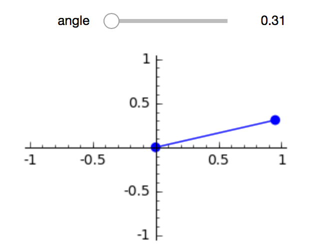
Fig. 86 The slider of the interact drives a crank.
Computing Coordinates of the Connector Point
There is a bar connected to the end point of the crank. The end point of that bar is connected to another bar, of length 5/2, that originates at (2,0). To find the coordinates of the connector point, we intersect two circles.
PR.<x,y,c,s> = PolynomialRing(QQ, order='lex')
p = (x-c)^2 + (y-s)^2 - (5/2)^2
q = (x-2)^2 + y^2 - (5/2)^2
print('p = ', p)
print('q = ', q)
With the resultant we get symbolic values for the coordinates, in function of the end point coordinates (c, s) of the crank.
ry = p.resultant(q,x)
rx = p.resultant(q,y)
print(ry)
print(rx)
To solve the polynomials for x and y, we must convert back to the Symbolic Ring (SR).
x, y, c, s = var('x,y,c,s')
sx = solve(SR(rx),x)
sy = solve(SR(ry),y)
print('sx = ', sx)
print('sy = ', sy)
We take the second solution as coordinates for x and the first solution for the coordinates for y. This was done by trial and error.
xv = sx[1].rhs()
yv = sy[0].rhs()
print('x = ', xv)
print('y = ', yv)
To use the formulas for the coordinates of the connector point, we make functions to substitute the arguments of the functions into the formulas for the coordinates of the connector point. These functions are used in our second interact.
fx(cs, sn) = xv.subs(c=cs, s=sn)
fy(cs, sn) = yv.subs(c=cs, s=sn)
@interact
def connector(angle = slider(0, 2*pi, 0.1, pi/2, label='angle')):
    """
    Shows the drawing of a crank, where the user can slide the angle
    to turn the crank.  Also the connector point is drawn.
    """
    center = (0,0)
    c = cos(angle)
    s = sin(angle)
    endpnt = (c, s)
    (x, y) = (fx(c,s), fy(c,s))
    pltcnt = point(center, size=50)
    pltend = point(endpnt, size=50)
    connector = point((x,y), size=50)
    crank = line([center, endpnt])
    bartwobase = point((2,0),size=50)
    bartwo = line([(2,0), (x,y)], color='red')
    barthree = line([endpnt, (x,y)], color='green')
    bars = crank + bartwo + barthree
    pnts = pltcnt + connector + pltend + bartwobase
    plt = bars + pnts
    plt.show(xmin=-1, xmax=3, ymin=-1, ymax=+3, figsize=3)
The result of the interact is shown in Fig. 87.
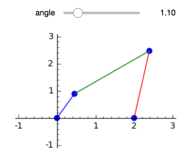
Fig. 87 An interact for a 4-bar mechanism, the slider drives the crank.
Adding the Coupler and Fourth Bar
The final addition is the coupler point and the fourth bar. The fourth bar lies in the extension of the end point of the crank and the connector point. As the fourth bar has the same length as the bar between the end point of the crank and the connector point, to obtain the coordinates of the coupler point, we add the differences between connector and end point of the crank to the coordinates of the connector point.
@interact
def coupler(angle = slider(0, 2*pi, 0.1, pi/2, label='angle')):
    """
    Shows the drawing of a crank, where the user can slide the angle
    to turn the crank.  Also the connector point is drawn,
    with the coupler point and fourth bar.
    """
    center = (0,0)
    c = cos(angle)
    s = sin(angle)
    endpnt = (c, s)
    (x, y) = (fx(c,s), fy(c,s))
    dx = x - c
    dy = y - s
    xx = x + dx
    yy = y + dy
    pltcnt = point(center, size=50)
    pltend = point(endpnt, size=50)
    connector = point((x,y), size=50)
    coupler = point((xx,yy), size=50, color='red')
    crank = line([center, endpnt])
    bartwobase = point((2,0),size=50)
    bartwo = line([(2,0), (x,y)], color='red')
    barthree = line([endpnt, (x,y)], color='green')
    barfour = line([(x,y), (xx,yy)], color='blue')
    bars = crank + bartwo + barthree + barfour
    pnts = pltcnt + connector + pltend + bartwobase + coupler
    plt = bars + pnts
    plt.show(xmin=-1, xmax=5, ymin=-1, ymax=+5, figsize=5)
As we move the crank, we see that the coupler point traces a straight line. Thus the mechanism translates the rotational motion of the crank to the straight motion of the coupler point. The result is shown in Fig. 85.
Deploying the Interactive Web Page
When we insert the code into a web page,
we must ensure that the entire context is defined.
For this application, this means that we declare the variables
c and s, and also define the formulas xv and yv.
Assignments
Add an extra parameter to the interact that shows the crank. The extra parameter is the length L of the crank, so the end point has coordinates (L*cos(angle), L*sin(angle)).
As a continuation of the previous exercise, find the coordinates of the connector point, symbolically in function of the variables c, s, and L.
Still as a continuation of the previous exercises, extend the interact of the connector with an extra slider for the length of the crank.
Finally, extend the interact of the coupler point with a slider for the length of the crank.
Extend the interact of the coupler point so that the path of the coupler point is drawn with a list_plot for the angle going from zero till the position determined by the current value of the angle.