Introduction

This first lecture outlines the course, describes our computational tools, and goes through four problems, solved by statistical reasoning.

Industrial Mathematics and Computation

The main goal of the course is to prepare for the solving of industrial problems.

Definition of Industrial Mathematics

Industrial Mathematics applies mathematics to solve problems in industry.

In this course, problems coming from science and government are interesting as well. The course is also a computational course. In particular, we pay attention to all aspects of applying software to solving problems.

Applying mathematics to solve problems involves three stages:

1. Model the problem as a mathematical problem.

2. Solve the mathematical problem.

3. Interpret the results in terms of the original problem.

The three stages may have to repeated for results to make sense.

In contrast to solving problems in academia, industrial problems center often around money and there are time constraints for a solution of the problem to arrive. Concerning time, it is important to be capable to make a first cut to have something to present before the closing of the business day.

Chapter 15 on Technical Writing by Craig Gunn, in the book of Charles R. MacCluer, opens with the sentence: You will be judged in industry not on your work but on how well you communicate your work. Communication includes technical writing and oral presentations of projects.

Julia and the Jupyter notebook

Julia is a relatively new programming language which combines the ease of a scripting language (such as Python) with the efficiency of a compiled language (such as C++). We use the Jupyter notebook to document our computations and describe the results. Jupyter stands for Julia, Python, R, and many others, and promotes language agnostic computing, as the Jupyter notebook supports many different languages.

The current stable version of Julia is 1.11.2 (December 1, 2024). Julia is free software. To install, do the following:

1. Visit <https://julialang.org>.

2. Install the Juliaup installation manager.

3. Adjust the path environment variable if needed.

There are two ways to run Julia:

1. in an interactive Terminal or PowerShell window; or

2. at the command prompt, type

   julia program.jl
   

   where program.jl is a Julia program.

The Jupyter notebook is a web based interface for computations.

• Cells can contain code or text.

• A well structured notebook can be printed as a technical report.

JupyterLab is the latest notebook environment.

To install the notebook with Julia, do the following:

1. In a Julia session, type using IJulia.

2. Answer y to download.

3. Type using Pkg; Pkg.build("IJulia").

4. Type using IJulia.

5. Type notebook().

The first time, the system will prompt you to install Jupyter.

Installing Julia and JupyterLab is the first, and one of the important exercises.

It is not good practice to install packages in a Jupyter notebook. Instead, open a terminal lauching the Julia prompt and type

using Plots

to install the Plots package. In solving one of the problems in one of the later subsections, we will also use the package QuadGK.

Random Variables, Expected Values, Variance

Selecting the most appropriate statistical distribution is often the key to solve a problem.

A random variable \(X\) models an experiment.

• \(P(X = x)\) is the probability that \(X\) takes the value \(x\).

• \(F(X \leq x)\) is the probability that \(X\) takes a value less than \(x\).

\(F\) is the cumulative probability distribution function:

\[P(a \leq X \leq b) = F(b) - F(a) = \int_a^b dF.\]

If \(F\) is differentiable, then \(f = F'\) is the density function.

Every random variable has an expected value, variance, and standard deviation, as defined below.

Definition of Expected Value and Variance.

A random variable \(X\) with cumulative probability density function \(F\) has expected value

\[\mu = E[X] = \int x dF\]

and variance

\[\sigma^2 = E[(X - \mu)^2].\]

The \(\sigma\) is the standard deviation of \(X\).

Four Problems, Four Distributions

To introduce the discrete uniform distribution, we consider the Rolling Dice Problem. We roll a fair 6-sided die ten times and ask the following questions:

• What is the expected value of the sum of the outcomes?

• What is the variation in the expected value?

In rolling a fair 6-sided die, every side has equal probability of \(\displaystyle \frac{1}{6}\).

• The mean value of one throw is 7/2, computed as

  \[\mu = 1 \left( \frac{1}{6} \right) + 2 \left( \frac{1}{6} \right) + 3 \left( \frac{1}{6} \right) + 4 \left( \frac{1}{6} \right) + 5 \left( \frac{1}{6} \right) + 6 \left( \frac{1}{6} \right) = 21/6.\]

This implies that after 10 rolls, we may expect the sum to be 35.

• The variance is \(35/12 \approx 2.9166\), computed as

  \[\sigma^2 = \frac{1}{6} \sum_{i=1}^6 \left( i - \frac{7}{2} \right)^2.\]

For one roll, we thus have \(3.5 \pm 2.9\). For ten rolls, we expect \(35 \pm 29\).

To introduce the normal distribution, we consider the Life Span Problem. Suppose a light bulb has an average life span of 1000 hours, with a standard deviation of 400 hours. Assuming a normal distribution, what is the probability that a bulb lasts 2000 hours or longer?

To answer this question, consider an example of the normal distribution, defined by the probability function

\[f(x) = \frac{1}{\sigma \sqrt{2 \pi}} e^{-(x-\mu)^2/2\sigma^2}, \mbox{ for } \mu = 1, \sigma = 0.4\]

The plot of \(f\) in Fig. 1 shows the bell shape of a probability distribution.

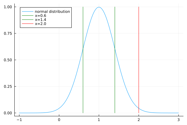
Fig. 1 The plot of a normal probability function \(f\).

The probability that a normally distributed random variable takes a value larger than 2 is expressed by

\[P(X > 2) = \int_2^\infty \frac{1}{\sigma \sqrt{2 \pi}} e^{-(x-\mu)^2/2\sigma^2} \quad \mbox{ for } \mu = 1, \sigma = 0.4\]

To evaluate this integral to compute the probability that our bulb lasts 2000 hours or longer, we use the package QuadGK in a Julia session, as illustrated below:

julia> using QuadGK

julia> f(x) = (1/(0.4*sqrt(2*pi)))*exp(-(x-1)^2/(2*0.4^2))
f (generic function with 1 method)

julia> val, err = quadgk(f, 0.6, 1.4, rtol=1.0e-8)
(0.682689492137086, 9.098977127308672e-11)

julia> val, err = quadgk(f, 2.0, 100.0, rtol=1.0e-8)
(0.006209665325776137, 2.981577782577757e-12)

The probability that a light bulb last 2000 hours or longer is 0.0062.

To introduce the binomial distribution, we consider the Staffing Problem. On average, for every three staffers who are emailed for a shift, only one shows up. How many staffers must be emailed to guarantee at least 20 show up, with a confidence of 90 per cent?

In applying the binomial distribution, observe, \(1/3 = p\) is the probability of a presence. Of \(n\) emails sent, the probability that \(k\) are present is

\[\begin{split}p(k) = \left( \begin{array}{c} n \\ k \end{array} \right) p^k (1 - p)^k,\end{split}\]

where the factor \(\displaystyle \left( \begin{array}{c} n \\ k \end{array} \right)\) equals all subsets of size \(k\) out of a total of \(n\).

Finding \(n\) so that the probability that less than 20 are present is less than 10 per cent is equivalent to solving the following inequality:

\[\begin{split}\sum_{k=0}^{19} p(k) = \sum_{k=0}^{19} \left( \begin{array}{c} n \\ k \end{array} \right) \left( \frac{1}{3} \right)^k \left( \frac{2}{3} \right)^{n-k} < 0.1\end{split}\]

To evaluate \(\displaystyle \sum_{k=0}^{19} p(k) = \sum_{k=0}^{19} \left( \begin{array}{c} n \\ k \end{array} \right) \left( \frac{1}{3} \right)^k \left( \frac{2}{3} \right)^{n-k}\), we use Julia as a calculator, as below.

Big integer arithmetic is applied with the big(n) and big(k) in the definitions of c(n,k).

julia> c(n,k) = factorial(n)/(factorial(k)*factorial(n-k))
c (generic function with 1 method)

julia> f(n) = sum([c(big(n),big(k))*(1/3)^k*(2/3)^(n-k) for k=0:19])
f (generic function with 1 method)

julia> f(60)
0.4515887757895708918836755159195509913398442126529291861812108271657047651381413

julia> f(73)
0.1136505489356501711588450629052906713758444342467108865237287073849361752409797

julia> f(74)
0.09950717529629137197668084287380332801796993918620879724884986272908044207906067

At least 74 emails must be sent to have 20 present with 90 per cent confidence.

To introduce the Poisson distribution, we consider an instance of the Arrival Problem. If a market has 60 customers per hour on average, then what is the probability that more than 20 customers check out in one quarter hour?

Knowing that time is continuous, let the time unit be one quarter of an hour. The random variable \(X\) is the number of arrivals per quarter hour. On average, we have 15 customers per quarter hour. The Poisson distribution has parameter \(\lambda\) and average \(\mu = \lambda T\), where \(T\) is the time unit:

\[p(k) = \frac{(\lambda T)^k}{k!} e^{-\lambda T} \quad \mbox{ and } \quad F(x) = e^{-\lambda T} \sum_{k=0}^x \frac{(\lambda T)^k}{k!}\]

We have \(F(x) = P(X \leq x) = 1 - P(X > x)\), so we have to compute \(\displaystyle e^{-15} \sum_{k=0}^{20} \frac{15^k}{k!}\).

To solve this problem, we run the following Julia function.

"""
    A market has 60 customers per hour on average.
What is the probability that more than 20 customers
check out in one quarter hour?
"""
function arrival()
    q = 0           # sum of probabilities
    m = 20          # number of arrivals
    lT = 15         # arrivals per quarter hour is lambda*T
    p = 1           # accumulates the product
    for k=1:m
        p = p*lT/k  # update the product
        q = q + p   # update the sum
    end
    q = q*exp(-lT)  # normalization
    p = 1 - q
    println("probability : ", p)
end

Running arrival() prints probability : 0.08297121593378054.

Exercises

0. Install Julia and the Jupyter notebook on your computer.

1. In Julia, rand((1,2,3,4,5,6)) simulates the roll of a 6-sided die. Run 1000 simulations of rolling a pair of 6-sided dice.

   1. How many times did \(2, 3, 4, \ldots, 12\) occur? Make a histogram of the sum of the outcomes.

   2. Graph the cumulative distribution function \(F(x)\).

2. Your friend asks your advice on a planned motor bike trip of 1,000 miles through the desert. Because of the rough terrain, tires are expected to last 1,500 miles with a standard deviation of 300 miles. As soon as one tire expires, the trip is over. What is the probability your friend gets stranded in the desert?

3. Suppose, on average, five percent of travelers do not show up or arrive too late to board the air plane. A flight is oversold if there are more tickets sold than the number of available seats on the plane. What is the percentage of the number of available seats that can be oversold and still give every traveler who shows up on time a seat?

4. Consider evaluating \(\displaystyle e^{-15} \sum_{k=0}^{20} \frac{15^k}{k!}\) with an array comprehension.

   1. Give the code for the array comprehension in Julia, with the default 64-bit floating-point arithmetic.

   2. Explain why the numerical value of the comprehension differs from the output of the function arrival.

   3. Use computer algebra to compute the exact value.

Bibliography

1. J. Bezanson, A. Edelman, S. Karpinski, and V. B. Shah. A Fresh Approach to Numerical Computing. SIAM Review, Vol 59, No 1, pages 65-98, 2017.

2. C. Forber, M. Evans, N. Hastings, and B. Peacock: Statistical Distributions. Fourth edition, John Wiley and Sons, 2011.

3. T. Kluyver, B. Ragan-Kelley, F. Perez, B. Granger, M. Bussonnier, J. Frederic, K. Kelley, J. Hamrick, J. Grout, S. Corlay, P. Ivanov, D. Avila, S. Abdalla, C. Willing, and Jupyter Development Team. Jupyter Notebooks—a publishing format for reproducible computational workflows. In F. Loizides and B. Schmidt, editors, Positioning and Power in Academic Publishing: Players, Agents, and Agendas, pages 87-90. IOS Press, 2016.

4. C. R. MacCluer: Industrial Mathematics. Modeling in Industry, Science, and Government. Prentice Hall, 2000.