Taguchi Quality Control

In the first part of the lecture, the control of quality is introduced, following the ideas of Taguchi. The second part introduces the orthogonality to study the factors influencing quality.

Quality Loss Function and Expected Loss

Let us start making some obvious points about what quality is not.

• Product quality is not product quantity.

  This is a cultural issue. The U.S. is a typical throw-away society with a diverse market, whereas Japan is a homogeneous society. The outcome of world war II promoted mass production and consumption in the U.S., while Japan suffered.

• Quality is not value.

  Value is subjective and related to the supply-demand-marketing chain. An object (like a worn out teddy bear) can have a tremendous personal value, but no quality.

Definition of Quality (Genichi Taguchi, 1986)

An article of good quality performs its intended functions without variability, and causes little loss through harmful side effects, including the cost of using it.

In order to understand this definition, we look closer at the three emphasized items in the sentence of the definition.

1. The key point is without variability.

   Prior to the ideas of Taguchi, people tought the production was okay as long as the products were within the tolerances. The reduction of variability is the goal of Taguchi quality control.

2. To enhance the quality we want to reduce loss.

   But we only care about loss caused by variability in the product, not by loss caused by harmful side effects. Consider for example liquor. The quality of a bottle of liquor is its percentage of alcohol, because its intended effect is intoxication. Harmful side effects are the accidents or fights, etc…

3. Modeling the loss by a quality loss function is central.

To introduce the quality loss function, consider for example the production of shirts, measured by neck size.

Let \(y\) be the size of the produced shirt, i.e.: its neck size; and \(m\) the buyer’s exact neck size.

We denote by \(L(y)\) the loss due to the difference between \(y\) and \(m\).

• When \(y < m\) (the shirt is too small), return (or discard) the item.

• When \(y > m\) (the shirt is too wide), we have to tailor.

Consider the mathematical Taylor expansion of \(L(y)\) about \(m\):

\[L(y) = L(m) + \frac{L'(m)}{1!} (y-m) + \frac{L''(m)}{2!} (y-m)^2 + {\rm higher~order~terms}.\]

Why does \(L(y)\) model the loss well? Consider:

• \(L(m) = 0\), if \(y\) equals \(m\), the neck size, then there is no loss.

• \(L'(m) = 0\), the loss is minimal for \(y=m\).

So, we may represent the loss by

\[L(y) \approx k (y-m)^2, \quad {\rm for~some~constant~} k.\]

The constant \(k\) is determined by interpolation, as we illustrate next by a numerical example.

Suppose the critical deviation from \(m\)

• for the shirt being too small occurs at \(\Delta m^- = 0.5\) cm,

• with corresponding cost of rejection being \(L^- = \$40\).

Furthermore, the shirt is found too wide

• when it deviates more than one cm from \(m\), i.e., \(\Delta m^+ = 1\) cm,

• with an associated cost for tailoring set at \(L^+ = \$20\).

Since we have different losses when too small or too wide, our quality loss function is piecewise quadratic:

\[\begin{split}L(y) = \left\{ \begin{array}{ll} k^+ (y-m)^2 & \mbox{ for } y \geq m, \\ k^- (y-m)^2 & \mbox{ for } y < m. \\ \end{array} \right.\end{split}\]

With critical deviations and corresponding costs:

• When a shirt is too small: \(\Delta m^- = 0.5\) cm, \(L^- = \$40\).

• When a shirt is too wide: \(\Delta m^+ = 1\) cm, \(L^+ = \$20\).

We determine \(k^+\) as follows (\(\Delta m^+ = y - m, y \geq m\)):

\[L^+ = k^+ ( \Delta m^+ )^2 \Rightarrow 20 = k^+ ( 1.0 )^2 \Rightarrow k^+ = 20.\]

Similarly, \(k^-\) is computed as follows (\(\Delta m^- = m - y, y < m\)):

\[L^- = k^- ( \Delta m^- )^2 \Rightarrow 40 = k^- ( 0.5 )^2 \Rightarrow k^- = 160.\]

The complete, numerical piecewise quality loss function is then, for \(m = 40\) cm, the neck size of the buyer:

\[\begin{split}L(y) = \left\{ \begin{array}{ll} 20 & \mbox{ for } y \geq 41 \\ 20(y - 40)^2 & \mbox{ for } 40 \leq y < 41 \\ 160(y - 40)^2 & \mbox{ for } 39.5 < y < 41 \\ 40 & \mbox{ for } y \leq 39.5 \\ \end{array} \right.\end{split}\]

which is encode in a function loss, in the syntax of the Julia language:

function loss(y)
    if y >= 41                 # $20 cost for too wide
        return 20
    elseif y >= 40
        return 20*(y-40)^2
    elseif y > 39.5
        return 160*(y-40)^2
    else                       # $40 cost for too small
        return 40
    end
end

The function loss is used to make the plot shown in Fig. 2. We observe that missing the target causses loss.

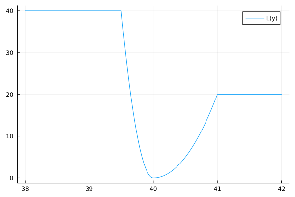
Fig. 2 The plot of a quality loss function \(L(y)\).

After this numerical example, we are ready for the general definition of the quality loss function.

Definition of quality loss function.

Denote by \(X\) the random variable modeling the outcome of production. Let \(\theta\) denote the target value for the production. Then the quality loss function is

\[L(X,\theta) = k (X-\theta)^2, \quad \mbox{for some constant } k.\]

We call the constant \(k\) the loss coefficient.

The cumulative probability distribution function is denoted by \(F(x)\),

• with mean \(\mu = E[X]\) and

• standard deviation \(\sigma^2 = E[(X-\mu)^2]\).

Given \(\mu\) and \(\sigma\), what is the expected loss?

Given a quality loss function \(L\), the expected loss \(E[L(X,\theta)]\) is derived below.

\[\begin{split}\begin{array}{rcl} E[L(X,\theta)] & = & {\displaystyle \int_{-\infty}^{+\infty} k (x - \theta)^2 d F(x)} \\ & = & {\displaystyle \int_{-\infty}^{+\infty} k (x - \mu + \mu - \theta)^2 d F(x)} \\ & = & {\displaystyle \int_{-\infty}^{+\infty} k [(x - \mu) + (\mu - \theta)]^2 d F(x)} \\ & = & {\displaystyle \int_{-\infty}^{+\infty} k (x - \mu)^2 d F(x) + \int_{-\infty}^{+\infty} 2 k (x - \mu)(\mu - \theta) d F(x)} \\ & & {\displaystyle +~ \int_{-\infty}^{+\infty} k (\mu - \theta)^2 d F(x)} \\ & = & {\displaystyle k \int_{-\infty}^{+\infty} (x - \mu)^2 d F(x)} \\ & & {\displaystyle +~ 2 k (\mu - \theta) \left( \int_{-\infty}^{+\infty} x dF(x) - \mu \int_{-\infty}^{+\infty} dF(x) \right)} \\ & & {\displaystyle +~ k (\mu -\theta)^2 \int_{-\infty}^{+\infty} d F(x)} \end{array}\end{split}\]

The above terms in the expected loss are simplified, introducing the following notations:

\[\sigma^2 = \int_{-\infty}^{+\infty} (x - \mu)^2 d F(x), \mu = \int_{-\infty}^{+\infty} x d F(x), \mbox{ and } \int_{-\infty}^{+\infty} d F(x) = 1,\]

into the following:

\[\begin{split}\begin{array}{rcl} E[L(X,\theta)] & = & {\displaystyle k \sigma^2 + 2 k (\mu -\theta) \left( \mu - \mu \right) + k (\mu -\theta)^2} \\ & = & {\displaystyle k \sigma^2 + k (\mu -\theta)^2} \end{array}\end{split}\]

The expected loss consists of two terms:

• the loss due to variability \(k \sigma^2\) and

• \(k (\mu -\theta)^2\) is the loss due to missing the target.

The derivation justifies the following definition of expected loss of quality.

Definition of Expected Loss.

Let \(L(X) = k (X - \theta)^2\) be the quality loss function, where

• \(k\) is the loss coefficient,

• \(\theta\) is the target value of the production,

• \(X\) is a random variable which models the production, with

  1. \(\mu = E[X]\), the mean value of the production,

  2. \(\sigma^2 = E[(X-\mu)^2]\), the standard deviation.

The expected loss is \(E[L(X,\theta)] = k \sigma^2 + k (\mu -\theta)^2\).

In an example on the cost of variance, we consider the color density of televisions.

The loss coefficient \(k\) is \(\$1.25\), so \(L(y) = 1.25(y - m)^2\), where \(y\) is the produced color density, \(m\) is the target color density. The expected loss is \(1.25 ( \sigma^2 + (\mu - m)^2 )\).

For televisions produced in San Diego and Tokyo, \(\mu - m = 0\), but

• \(\sigma^2 = 8.33\) for the San Diego plant, and

• \(\sigma^2 = 2.78\) for the Tokyo plant.

The expected loss per television is then computed as

• \(1.25 ( 8.33 + 0) = \$10.41\) per unit for the San Diego plant, and

• \(1.25 ( 2.78 + 0) = \$3.48\) per unit for the Tokyo plant.

Even as both plants have the same averages of their production, the larger deviation at the San Diego plant makes for a larger expected loss than at the Tokyo plant.

Factor Analysis

The quality of a product is influenced by many factors. Trying all combinations of the factor is too costly. Factor analysis reduces the number of experiments needed to improve the product quality.

Which factors have the most effect on quality? Examining a production line, we could do better

• if only we had better machines,

• if only we had better trained people,

• if only we had more production time,

• …

Of the factors listed above, which is most important? How do we relate the factors to quality?

To introduce a solution for this problem, suppose we have three factors \(x_1\), \(x_2\), \(x_3\). Let \(L(x_1,x_2,x_3)\) denote the loss of quality as a function of the three factors. Then we apply Taylor expansion again and use a linear approximation:

\[L(x_1,x_2,x_3) = \alpha_0 + \alpha_1 x_1 + \alpha_2 x_2 + \alpha_3 x_3.\]

Then, the factor with the largest coefficient has the largest impact. So, our problem is reduced to determining the coefficients \(\alpha_1\), \(\alpha_2\), and \(\alpha_3\). To determine the coefficients, we can run the production many times, for

\[-1 \leq x_i \leq +1, \quad i=1,2,3,\]

setting each factor once low (\(-1\)) and once high (\(+1\)).

For example:

\[\begin{split}\begin{array}{rcl} - L(-1, x_2 = c_2, x_3 = c_3 ) & = & \alpha_0 - \alpha_1 + \alpha_2 c_2 + \alpha_3 c_3 \\ + L(+1, x_2 = c_2, x_3 = c_3 ) & = & \alpha_0 + \alpha_1 + \alpha_2 c_2 + \alpha_3 c_3 \\ \cline{1-3} L(+1, x_2 = c_2, x_3 = c_3 ) & = & 2 \alpha_1 \end{array}\end{split}\]

While effective, the main problem is that \(2^3 = 8\) runs are needed, for three factors. The number of runs grows exponentially in the number of factors.

The number of runs can be reduced dramatically by an orthogonal array of experiments. We run four experiments and observe \(L_1\), \(L_2\), \(L_3\), \(L_4\), as follows:

\[\begin{split}\begin{array}{ccccc} & x_1 & x_2 & x_3 & \\ \hline 1: & +1 & -1 & -1 & L_1 \\ 2: & -1 & +1 & -1 & L_2 \\ 3: & +1 & +1 & +1 & L_3 \\ 4: & -1 & -1 & +1 & L_4 \end{array}\end{split}\]

Observe: (1) Every column sums up to zero. (2) The inner product of every column with every other column is zero. We say that the columns are orthogonal to each other.

How this improve the solution to our problem? Well, we apply linear algebra. First, apply the array to

\[L(x_1,x_2,x_3) = \alpha_0 + \alpha_1 x_1 + \alpha_2 x_2 + \alpha_3 x_3\]

to obtain

\[\begin{split}\begin{array}{rclcl} L(+1, -1, -1) & = & \alpha_0 + \alpha_1 - \alpha_2 - \alpha_3 & = & L_1 \\ L(-1, +1, -1) & = & \alpha_0 - \alpha_1 + \alpha_2 - \alpha_3 & = & L_2 \\ L(+1, -1, +1) & = & \alpha_0 + \alpha_1 - \alpha_2 + \alpha_3 & = & L_3 \\ L(-1, +1, +1) & = & \alpha_0 - \alpha_1 + \alpha_2 + \alpha_3 & = & L_4 \\ \cline{1-3} & & 4 \alpha_0 & = & L_1 + L_2 + L_3 + L_4 \end{array}\end{split}\]

In matrix-vector notation:

\[\begin{split}\left[ \begin{array}{ccc} +1 & -1 & -1 \\ -1 & +1 & -1 \\ +1 & -1 & +1 \\ -1 & +1 & +1 \end{array} \right] \left[ \begin{array}{c} \alpha_1 \\ \alpha_2 \\ \alpha_3 \end{array} \right] = \left[ \begin{array}{c} L_1 - \alpha_0 \\ L_2 - \alpha_0 \\ L_3 - \alpha_0 \\ L_4 - \alpha_0 \end{array} \right].\end{split}\]

The solution of a linear system simplifies greatly when the matrix is orthogonal. In matrix-vector notation, \(A {\boldsymbol \alpha} = {\bf b}\):

\[\begin{split}A = \left[ \begin{array}{ccc} +1 & -1 & -1 \\ -1 & +1 & -1 \\ +1 & -1 & +1 \\ -1 & +1 & +1 \end{array} \right], \quad {\boldsymbol \alpha} = \left[ \begin{array}{c} \alpha_1 \\ \alpha_2 \\ \alpha_3 \end{array} \right], \quad {\bf b} = \left[ \begin{array}{c} L_1 - \alpha_0 \\ L_2 - \alpha_0 \\ L_3 - \alpha_0 \\ L_4 - \alpha_0 \end{array} \right].\end{split}\]

By the orthogonality: \(A^T A = 4 I\), where \(I\) is the identity matrix. So we simply read off the values for \(\boldsymbol \alpha\) from \(A^T {\bf b}\).

Exercises

1. Suppose an item costs \(\$117\) to manufacture. If the item misses the target of 12 by a margin of 3, then the item must be discarded. The production has a mean of 11.7 and standard deviation of 1.0.

   1. Determine the quality loss function.

   2. Suppose an effort of \(\$20\) per item reduces the standard deviation to 0.95. Is this a worthwhile effort?

2. Under normal circumstances, a tire has an expected life span of 80,000 miles.

   A car maintenance shop keeper has the choice between two different types of tires, we call them \(A\) and \(B\). A tire of type \(A\) costs \(\$200\) and has an average life span of 85,000 miles with a standard deviation of 10,000 miles. Type \(B\) sells for \(\$220\) and lasts 81,000 miles on average, with a standard deviation of 2,000 miles.

   1. Which type of tire has the best quality?

   2. Keeping the price of tire \(A\) fixed at \(\$200\), determine the price of tire \(B\) so both \(A\) and \(B\) have the same quality.

3. Construct a 9-by-4 orthogonal array using an equal amount of \(-1\), \(0\), and \(+1\) per column.

   • The sum of the element in each column is zero, and

   • the columns are orthogonal to each other.

   Explain your work.

Bibliography

• G. Taguchi. Introduction to Quality Engineering. Designing Quality into Products and Processes. Asian Productivity Organization, 1986.

• Handbook of Total Quality Management, edited by Christian N. Madu. Springer-Verlag, 1998.