The Monte Carlo Method
The expected value of a simulation can be expressed as a definite integral in several values, but often this integral is too complicated to evaluate exactly and can only be estimated.
Expected Values
To introduce the Monte Carlo method, consider a simulation to estimate \(\pi\). In Fig. 3 is the geometric interpretation of \(\pi/4\), and its expression as a definite integral.
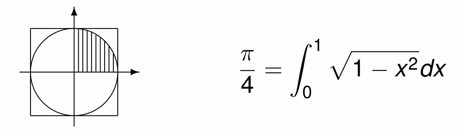
Fig. 3 The area of the unit disk and the integral for \(\pi/4\).
There are two steps in the simulation algorithm to estimate \(\pi\).
Generate random uniformly distributed points with coordinates
\[(x,y) \in [-1,+1] \times [-1,+1].\]We count the generated \((x,y)\) as a success when \(x^2 + y^2 \leq 1\).
Then \(\displaystyle \pi \approx \frac{\mbox{total number of successes}} {\mbox{total number of trials}}\).
The development of the code for the simulation algorithms
starts with some interactive experiments.
In Julia, the command rand(10) returns a vector
of 10 random numbers in \([0,1]\).
One million points are generated in the session below:
julia> N = 10^7;

julia> x = rand(N); y = rand(N);

julia> z = x.^2 + y.^2;

julia> 4*sum([Int32(t <= 1.0) for t in z])/N
3.1418236
We observe the following.
The semicolon
;suppresses the output.The dot before the exponent is for a componentwise operation.
The True/False is converted to 1/0 by
Int32(t <= 1.0).
The performance of the interactive experiments could improve, as it requires to keep the three vectors of a million numbers in main memory. Improving memory consumption is left as an exercise.
We apply the Monte Carlo method to solve the Newsboy Problem, starting with a numerical example of this problem. A newspaper seller has on average 100 customers a day as 5000 people are passing by the shop each day. The seller has to buy each paper at 50 cents a copy, sells it at 75 cents, with no returns. For each sold paper, the seller makes a profit of 25 cents, the loss is 75 cents for each unsold paper. To maximize profit, how many copies should the seller buy?
The sentence A newspaper seller has on average 100 customers a day as 5000 people are passing by the shop each day. translates into the following simulation:
Flip a loaded coin (with probability 100/5000) five thousand times, say that heads comes up with probability 1/50.
Count each head as a one, as a customer who buys a paper.
How many copies should the seller buy? Run the simulation starting with 90, then 91, 92, 93, \(\ldots\), to 110 and for each run, compute the profit. Take the average for 365 days, for 365 simulations.
Julia code for this simulation is listed next:
function newsboy()
    (maxprofit, maxidx) = (0, 0)
    for nbpapers = 90:110
        sumday = 0
        for day=1:365
            profit = -nbpapers*0.50
            nbsold = 0
            for passerby=1:5000
                if nbsold < nbpapers
                    if rand() <= 1.0/50
                        profit = profit + 0.75
                        nbsold = nbsold + 1
                    end
                end
            end
            sumday = sumday + profit
        end
        avgday = sumday/365
        println("profit from ", nbpapers, " : \$", avgday)
        if maxprofit < avgday
            maxprofit = avgday
            maxidx = nbpapers
        end
    end
    print(" maximum profit : \$", maxprofit)
    println(" at ", maxidx)
end
The output of a run in a terminal window follows:
$ julia newsboy.jl
profit from 90 : $21.94
profit from 91 : $22.23
profit from 92 : $22.05
profit from 93 : $22.35
profit from 94 : $22.17
profit from 95 : $22.38
profit from 96 : $22.52
profit from 97 : $22.16
profit from 98 : $22.22
profit from 99 : $21.72
profit from 100 : $22.24
profit from 101 : $21.92
profit from 102 : $22.11
profit from 103 : $21.43
profit from 104 : $21.23
profit from 105 : $21.43
profit from 106 : $20.98
profit from 107 : $20.12
profit from 108 : $20.14
profit from 109 : $19.53
profit from 110 : $19.26
 maximum profit : $22.52 at 96
Profit is maximized at \(\$22.52\) when the newsboy has bought 96 copies of the paper. Observe that the simulation is executed for only 365 days, which is actually a small sample size, leading to inaccurate estimates. It is better to run over longer time spans and not only average the results, but also to compute the variance.
Mean Time Between Failures
We consider the life span of a multi-component product. In particular, given is a composite product of \(n\) components:
The life span of the i-th component is normally distributed with mean \(\mu_i\) and standard deviation \(\sigma_i\), for \(i=1,2,\ldots,n\).
The composite product fails if any of its components fails.
What is the average life span of the composite product?
To answer this question, we apply a simulation algorithm, formulated below.
Using pseudo code, the simulation algorithm can be described as below.
sum := 0
for i from 1 to N do
    t[j] is j-th sample of T[i]
end for
sum := sum + min(t[1], t[2], .., t[n])
report sum/N
This algorithm estimates an \(n\)-dimensional integral.
The specification of a Julia function to implement the simulation algorithm is below, starting with the documentation string of the function.
"""
    mtbf(means::Vector{Float64},
         deviations::Vector{Float64},
         N::Int,
         verbose::Bool=false)

returns the expected lifespan and the standard deviation
of a multicomponent product, given the means and standard
deviations of its components in the two vectors on input,
using N trials in the simulation.

If verbose, then each sample is written.
"""
The definition of the function follows next:
function mtbf(means::Vector{Float64},
              deviations::Vector{Float64}, N::Int,
              verbose::Bool=false)
   (m1, m2) = (0, 0)                       # moments
   sample = [0.0 for j=1:length(means)]    # work space
   for i=1:N                               # run N simulations
       for j=1:length(means)
           sample[j] = means[j] + deviations[j]*randn()
       end
       if verbose                          # for debugging
           println("sample : ", sample)
       end
       lifespan = minimum(sample)
       m1 = m1 + lifespan/N                # update the average
       m2 = m2 + lifespan*lifespan/N       # update second moment
   end
   return (m1, sqrt(m2 - m1*m1))           # mean and deviation
end
The randn() has a mean of zero and standard deviation of one.
In running a simulation, assume we have three components:
The means are 11, 12, and 13.
The standard deviations are 1, 2, and 3.
Let us take 10,000 samples in a simulation. The output of running a simulation with those parameters is listed below:
expected life span : 10.099215794814308
standard deviation : 1.371475210671779
as a result of the statements:
(mu, sigma) = mtbf([11.0, 12.0, 13.0], [1.0, 2.0, 3.0], 10000)
println("expected life span : ", mu)
println("standard deviation : ", sigma)
It is important to realize that the accuracy is only about one or at most two decimal places…
Normal bodies have two kidneys, two lungs, two eyes, … As an exercise, consider the lifespan with backup components.
Servicing Requests
How long does it take to service a sequence of requests, given the distribution of the arrival and service times?
Our problem is to predict the checkout time in a store. This time depends on three parameters:
arrival times of jobs,
service times to handle requests,
number of processors.
In our model for checkout lines, to estimate the wait times, we use the following distributions:
Arrival times are modeled by the Poisson distribution.
The service times depend on the size of each job, which we assume to follow a uniform or normal distribution.
The Poisson distribution depends on the parameter \(\lambda > 0\), be a positive real number, where \(\lambda\) is the expected number of events in a time interval assuming events occur independently. The probability that exactly \(k\) events happen is then:
By definition, the mean, or average, is \(\lambda\), the standard deviation is \(\sqrt{\lambda}\).
To generate random numbers, following a Poisson distribution, the following algorithm from The Art of Computer Programming, volume 2 Seminumerical Algorithms, (3rd edition, 1998; page 137) by Donald E. Knuth can be applied.
Input: \(\lambda\), average number of events per time interval.
Output: \(N\), number of events per time interval.
Given a uniform random number generator, the algorithm to generate numbers along the Poisson distribution can be written in pseudo code as follows:
L := exp(-lambda); k := 0; p := 1
do
   k := k + 1
   draw u in [0, 1] at random
   p := p * u
while ( p > L )
N := k - 1
At its core, the algorithm applies a uniform random number generator.
The Poisson distribution is available to Julia programmers
via the package StatsKit as illustrated in a command line
session below.
julia> using StatsKit

julia> p = Poisson(10)
Poisson{Float64}(?=10.0)

julia> rand(p, 10)
10-element Vector{Int64}:
  8
 11
  5
 11
  6
 11
 11
 12
  9
 11

julia>
The 10-element vector represents 10 random arrival times where the average number of arrivals equals 10 as well.
The flowchart for the simulation is shown in Fig. 4.
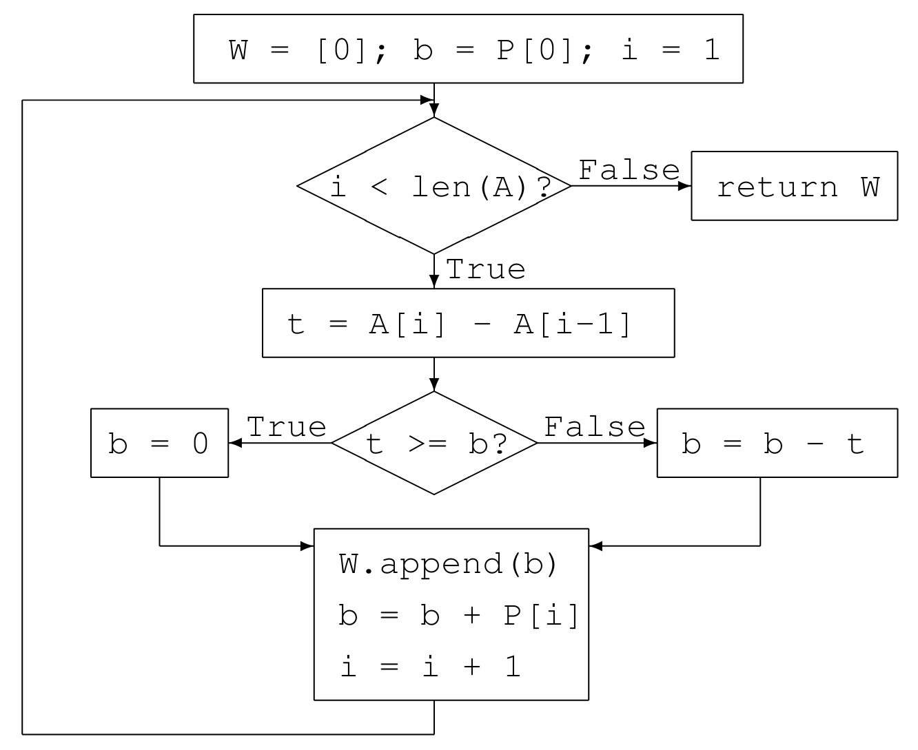
Fig. 4 Flowchart to compute the wait times in a checkout line.
To setup the simulation, we have to specify three parameters:
The number of arrivals per time step: \(\lambda\).
The maximum number of items for each job: \(M\).
The speed of the processor: time to process one item.
If there are 4 arrivals in one time step, then there arrival times are 0.0, 0.25, 0.50, 0.75, simulating the queuing of arrivals, one after the other. The setup function generates two vectors of the same size:
The arrival times of the jobs.
The sizes of the jobs.
The flowchart in Fig. 4 is encoded in the Julia function below.
"""
    process_requests(arrivals::Vector{Float64},
                     jobs::Vector{Int}, speed::Float64)

returns the waiting times for the jobs
with given arrival times and sizes.
"""
function process_requests(arrivals::Vector{Float64},
                          jobs::Vector{Int}, speed::Float64)
   wait = [0.0 for i=1:length(arrivals)]
   busy = jobs[1]*speed
   for i=2:length(arrivals)
       elapsed = arrivals[i] - arrivals[i-1]
       if elapsed >= busy
           busy = 0
       else
           busy = busy - elapsed
       end
       wait[i] = busy
       busy = busy + jobs[i]*speed
   end
   return wait
end
The output of one run, at the command line, is below:
$ julia estimatewait.jl
Lambda : 10, max#items : 7, speed : 0.02.
Simulation with 1000 trials :
 the average wait time : 0.13
the standard deviation : 0.21
The servicing requests problem also models client/server interactions. Servers are multithreaded: we consider multiple processors in the fifth exercise.
Exercises
For the estimation of \(\pi\), take
Nequal to \(10^8\), \(10^9\), etc.What are the resources in memory and time for increasing
N?How many decimal places in \(\pi\) do we gain as
Nincreases?Rewrite the simulation so that not all points are in memory.
Redo the experiments for increasing
N. Report the improvements.A grocery store has a bake shop. A loaf of bread costs 90 cents to make.
When fresh, sold on the same day, it sells for \(\$1.40\).
The next day, the loaf sells for 70 cents.
After two days, the loaf has to be discarded.
Given that of the 300 customers in the store, on average 20 customers buy a loaf of bread. To maximize profit, how many loaves of bread should the shop bake?
Justify your answer by adapting the simulation for the newsboy problem.
Use
randn()to generate one million random numbers.How many of those generated numbers lie in \([-1,+1]\)? Is this normal?
Approximating the cumulative distribution function, count how many of the generated numbers are less than \(-3 + 0.1 k\), for \(k\) ranging from 0 to 60, making 61 counts.
Apply simulation to estimate the life span of a multicomponent product with backups, to answer the following:
The product has three components, all with mean 10 and standard deviation 1.
The second component is a backup of the first. For the product to fail:
the first two components both fail, or
the third component fails.
Estimate the life span and standard deviation with at least 10,000 samples in a simulation.
Describe a modification to the servicing requests problem:
There are \(m\) processors, all operating at the same speed.
If there is no idle processor, then the job is rejected.
Instead of the waiting time, the modified simulation counts the number of rejected jobs.