Z-Transforms and Linear Recursions

The motivating problem for this lecture goes as follows.

• A train leaves the depot empty.

• At each station, on average, 40 people mount, while 20% of the riders dismount.

Suppose we are consultants for a train company, who asks us: Will there ever be a train long enough to accommodate the 40 people mounting at each station?

Signal Processing

Introducing signal processing, consider the schematic for a data acquisition system in Fig. 9.

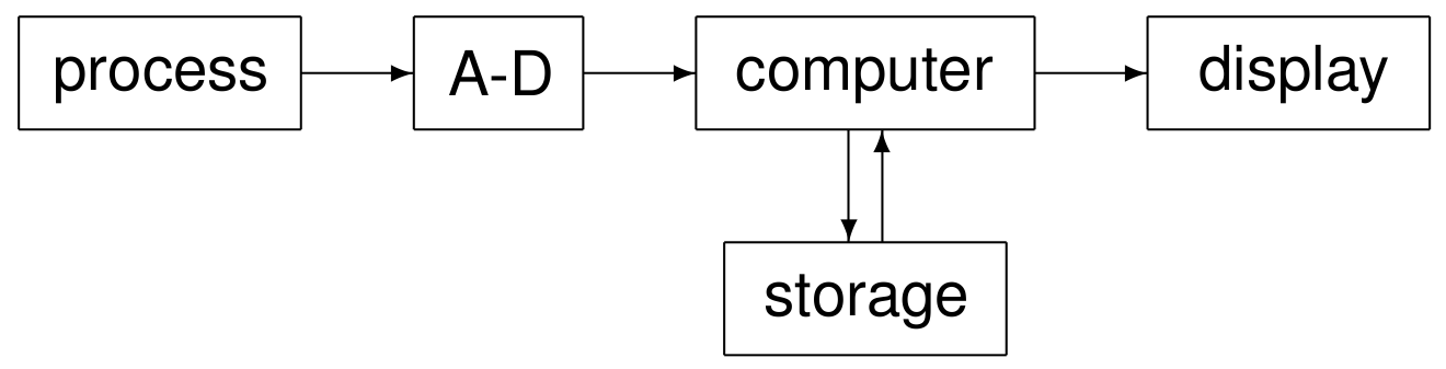
Fig. 9 Schematic of a data acquisition system.

The data acquisition process has three stages:

1. A process is measured by a sensor.

2. The measurements are converted from analog to digital (A-D).

3. The computer manipulates, stores, and displays the data.

We are concerned with the third stage of the acquisition process.

The Z-Transform of a signal

To introduce the z-transform of a signal, consider Fig. 10.

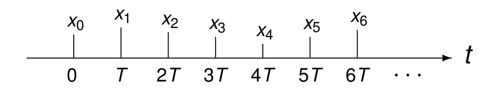
Fig. 10 Every \(T\) time units, a signal is sampled.

Definition of the z-transform of a signal.

The samples of the signal define a sequence \(x\) in the time domain:

\[x = \{ x_0, x_1, x_2, x_3, x_4, x_5, x_6, \ldots \}.\]

In the frequency domain, we define the Laurent series

\[X = \sum_{k=0}^\infty x_k z^{-k} = x_0 + \frac{x_1}{z} + \frac{x_2}{z^2} + \frac{x_3}{z^3} + \frac{x_4}{z^4} + \frac{x_5}{z^5} + \frac{x_6}{z^6} + \cdots\]

as the z-transform of the signal, as the series converges for \(|z| > 1\).

In studying signals, we are interested in capturing their growth or decay. As our first example, let us consider a constant signal. In the series

\[\frac{1}{1-z} = 1 + z + z^2 + z^3 + z^4 + z^5 + z^6 + \cdots\]

replace \(z\) by \(1/z\) to obtain:

\[\frac{1}{1-z^{-1}} = 1 + z^{-1} + z^{-2} + z^{-3} + z^{-4} + z^{-5} + z^{-6} + \cdots\]

So the z-transform of \(x = \{ 1, 1, 1, 1, 1, 1, 1, \ldots \}\) is

\[X = \frac{1}{1 - z^{-1}} = \frac{z}{z - 1}.\]

For any constant \(\alpha\), \(x = \{ \alpha, \alpha, \alpha, \ldots \}\) has z-transform \(\displaystyle X = \frac{\alpha z}{z-1}\).

Our second example has exponential growth. Again, in the series

\[\frac{1}{1-z} = 1 + z + z^2 + z^3 + z^4 + z^5 + z^6 + \cdots\]

replace \(z\) by \(2/z\) to obtain:

\[\frac{1}{1 - 2 z^{-1}} = 1 + 2 z^{-1} + 4 z^{-2} + 8 z^{-3} + 16 z^{-4} + 32 z^{-5} + 64 z^{-6} + \cdots\]

So the z-transform of \(x = \{ 1, 2, 4, 8, 16, 32, 64, \ldots \}\) is

\[X = \frac{1}{1 - 2 z^{-1}} = \frac{z}{z - 2}.\]

Observe: the essence of the signal, the growth rate is the root of \(z-2\).

Our third example has exponential decay. Once more, in the series

\[\frac{1}{1-z} = 1 + z + z^2 + z^3 + z^4 + z^5 + z^6 + \cdots\]

replace \(z\) by \(1/(2z)\) to obtain:

\[\frac{1}{1 - \frac{1}{2} z^{-1}} = 1 + \frac{1}{2} z^{-1} + \frac{1}{4} z^{-2} + \frac{1}{8} z^{-3} + \frac{1}{16} z^{-4} + \frac{1}{32} z^{-5} + \frac{1}{64} z^{-6} + \cdots\]

So the z-transform of \(\displaystyle x = \left\{ 1, \frac{1}{2}, \frac{1}{4}, \frac{1}{8}, \frac{1}{16}, \frac{1}{32}, \frac{1}{64}, \ldots \right\}\) is

\[X = \frac{1}{1 - \frac{1}{2} z^{-1}} = \frac{z}{z - \frac{1}{2}}.\]

The essence of the signal, the decay rate is the root of \(z-1/2\).

Delayed Signals and Weighted Averages

What is the z-transform of a delayed signal?

• Let \(x = \{ x_0, x_1, x_2, x_3, x_4, x_5, x_6, \ldots \}\) have z-transform \(\displaystyle X = \sum_{k=0}^\infty x_k z^{-k}\).

• Let \(y\) be the signal \(x\) with one time unit delay:

  \[y = \{ 0, x_0, x_1, x_2, x_3, x_4, x_5, x_6, \ldots \}.\]

What is the z-transform \(Y\) of \(y\)? Well, consider

\[X = \sum_{k=0}^\infty x_k z^{-k} = x_0 + \frac{x_1}{z} + \frac{x_2}{z^2} + \frac{x_3}{z^3} + \frac{x_4}{z^4} + \frac{x_5}{z^5} + \frac{x_6}{z^6} + \cdots\]

We then apply the definition of the z-transform:

\[Y = \frac{x_0}{z} + \frac{x_1}{z^2} + \frac{x_2}{z^3} + \frac{x_3}{z^4} + \frac{x_4}{z^5} + \frac{x_5}{z^6} + \frac{x_6}{z^7} + \cdots = z^{-1} X.\]

to find \(z^{-1} X\) as the z-transform of the delayed signal.

What is the z-transform of a weighted average?

• Let \(x\) be a signal with z-transform \(X\).

• Let us make a new signal \(y\), with a weighted average.

  \[y_k = \alpha x_k + \beta x_{k-1}, \quad \alpha + \beta = 1, \quad x_{-1} = 0.\]

What is the z-transform \(Y\) of \(y\)? We compute:

\[\begin{split}\begin{array}{rcl} Y & = & {\displaystyle \sum_{k=0}^\infty y_k z^{-k}} ~~=~~ {\displaystyle \sum_{k=0}^\infty \left( \vphantom{z^{-k}} \alpha x_k + \beta x_{k-1} \right) z^{-k}} \\ & = & {\displaystyle \sum_{k=0}^\infty \alpha x_k z^{-k} + \sum_{k=0}^\infty \beta x_{k-1} z^{-k}} \\ & = & \alpha X + \beta z^{-1} X ~~=~~ (\alpha + \beta z^{-1}) X. \end{array}\end{split}\]

Solving Linear Recursions by Z-Transforms

Recall our motivating problem:

• A train leaves the depot empty.

• At each station, on average, 40 people mount, while 20% of the riders dismount.

We can define a recursion relation for this problem:

1. Let \(x_n\) be the number of riders at the \(n\)-th station. \(x_0 = 0\), as the train leaves the depot empty.

2. As 20% dismount, 80% or 4 out of five remain, forty are added:

   \[x_n = \left( \frac{4}{5} \right) x_{n-1} + 40, \quad n = 1, 2, \ldots\]

With z-transforms we can solve linear recursions.

Definition of a linear recursion.

Given \(n\) fixed constants \(\alpha_1\), \(\alpha_2\), \(\ldots\), \(\alpha_n\), a linear recursion is

\[x_k = \alpha_1 x_{k-1} + \alpha_2 x_{k-2} + \cdots + \alpha_n x_{k-n},\]

where \(n\) initial values \(x_{-1}\), \(x_{-2}\), \(\ldots\), \(x_{-n}\) are known.

The general method to solve a linear recursion proceeds in three steps:

1. Transform the recursion to the frequency domain.

2. Solve the transformed recursion.

3. Transform the solution back to the time domain.

For our motivating problem, we derived the linear recursion:

\[x_n = \left( \frac{4}{5} \right) x_{n-1} + 40, \quad n = 1, 2, \ldots\]

The z-transform is

\[X = \left( \frac{4}{5} \right) z^{-1} X + 40 \frac{z}{z-1}.\]

We solve to obtain \(X\) as an expression in \(z\):

\[\left( 1 - \frac{4}{5} z^{-1} \right) X = 40 \frac{z}{z-1}\]

and find

\[X = \left( \frac{40z}{z-1} \right) \left( \frac{5z}{5z - 4} \right) = 200 \frac{z^2}{(z-1)(5z-4)}.\]

To process this answer further, we need the partial fraction decomposition.

Definition of the partial fraction decomposition.

Consider a quotient of two polynomials \(\displaystyle \frac{p(x)}{q(x)}\).

• Let \(q(x) = (x - \alpha_1)(x - \alpha_2) \cdots (x - \alpha_n)\) with mutually distinct roots: \(\alpha_i \not= \alpha_j\), for all \(i \not= j\).

• Let \(p(x)\) be any polynomial of degree \(\deg(p) < n\).

Then the partial fraction decomposition of the quotient is

\[\frac{p(x)}{q(x)} = \sum_{i=1}^n \frac{p(\alpha_i)}{q'(\alpha_i)} \left( \frac{1}{x-\alpha_i} \right).\]

Observe: \(\alpha_i \not= \alpha_j\), for all \(i \not= j\) implies \(q'(\alpha_i) \not = 0\).

For the proof of this rewriting of a quotient we apply Lagrange interpolation. The Lagrange form of the polynomial interpolating \(p(x)\) through \(\alpha_1\), \(\alpha_2\), \(\ldots\), \(\alpha_n\) is

\[\begin{split}p(x) = \sum_{i=1}^n p(\alpha_i) \prod_{\substack{j = 1 \\ j \not=i}}^n \left( \frac{x - \alpha_j}{\alpha_i - \alpha_j} \right).\end{split}\]

Because

• the interpolation problem has a unique solution, and

• \(\deg(p) < n\),

the Lagrange form of the interpolating polynomial equals \(p(x)\). Rewriting the Lagrange interpolating polynomial then goes as follows.

\[\begin{split}\begin{array}{rcl} p(x) & = & {\displaystyle \sum_{i=1}^n p(\alpha_i) \prod_{\substack{j = 1 \\ j \not=i}}^n \left( \frac{x - \alpha_j}{\alpha_i - \alpha_j} \right) \left( \frac{x - \alpha_i}{x - \alpha_i} \right)} \\ & \vphantom{{}_=^=} & \\ & = & {\displaystyle \sum_{i=1}^n \left( \frac{p(\alpha_i)}{x - \alpha_i} \right) \underbrace{ \prod_{j = 1}^n \left( \vphantom{\frac{1}{2}} x - \alpha_j \right) }_{q(x)} \prod_{\substack{j = 1 \\ j \not=i}}^n \left( \frac{1}{\alpha_i - \alpha_j} \right) } \\ {\displaystyle \frac{p(x)}{q(x)}} & = & {\displaystyle \sum_{i=1}^n \frac{p(\alpha_i)}{q'(\alpha_i)} \left( \frac{1}{x-\alpha_i} \right),} \end{array}\end{split}\]

as

\[\begin{split}\displaystyle q'(x) = \sum_{i=1}^n \prod_{\substack{j = 1 \\ j \not=i}}^n (x - \alpha_j).\end{split}\]

This completes the proof.

Returning now once more to our motivating problem, for the z-transform, we found:

\[X = 200 \frac{z^2}{(z-1)(5z-4)} = 40 z \frac{z}{(z-1)(z-4/5)}.\]

And then we apply

\[\frac{p(x)}{q(x)} = \sum_{i=1}^n \frac{p(\alpha_i)}{q'(\alpha_i)} \left( \frac{1}{x-\alpha_i} \right)\]

to find

\[\begin{split}\begin{array}{rcl} {\displaystyle \frac{z}{(z-1)(z-4/5)}} & = & {\displaystyle \frac{1}{q'(1)} \left( \frac{1}{z - 1} \right) + \frac{4/5}{q'(4/5)} \left( \frac{1}{z - 4/5} \right)} \\ & = & {\displaystyle 5 \left( \frac{1}{z - 1} \right) - 4 \left( \frac{1}{z - 4/5} \right).} \end{array}\end{split}\]

Then we arrive at the solution combining

\[X = 40 z \frac{z}{(z-1)(z-4/5)}\]

and

\[\frac{z}{(z-1)(z-4/5)} = 5 \left( \frac{1}{z - 1} \right) - 4 \left( \frac{1}{z - 4/5} \right)\]

which gives

\[X = 200 \left( \frac{z}{z-1} \right) - 160 \left( \frac{z}{z-4/5} \right) = 200 \left( \frac{z}{z-1} - \frac{(4/5)z}{z-4/5} \right).\]

Observe that we find 200 as an upper bound, which answers the original question.

For completeness, we bring the solution from the frequency domain into the time domain. We compute the inverse of

\[X = 200 \left( \underbrace{\frac{z}{z-1}}_{X_1} - \underbrace{\frac{(4/5)z}{z-4/5}}_{X_2} \right)\]

as follows:

1. Let \(x_1\) be the inverse of \(X_1\): \(x_1 = \{ 1, 1, 1, \ldots \}\).

2. Let \(x_2\) be the inverse of \(X_2\): \(\displaystyle x_2 = \frac{4}{5} \left\{ 1, \frac{4}{5}, \left( \frac{4}{5} \right)^2, \ldots \right\}\).

Now we make a linear combination:

\[x = \left\{ 1 - \frac{4}{5}, 1 - \left( \frac{4}{5} \right)^2, 1 - \left( \frac{4}{5} \right)^3, \ldots \right\}, \mbox{~or~} x_k = 200 \left( 1 - \left( \frac{4}{5} \right)^k \right),\]

for \(k= 1, 2, \ldots\), using the initial condition \(x_0 = 0\).

While our motivating problem was simple enough to be solved by hand, most problems are not that simple. Below is an interactive Julia session using sympy.rsolve to solve our recursion.

julia> using SymPy

julia> n = Sym("n")
n

julia> x = SymFunction("x")
x

julia> eq = Eq(x(n), (4/5)*x(n-1) + 40)
x(n) = 0.8x(n - 1) + 40

julia> init = Dict(x(0) => 0)
Dict{Sym, Int64} with 1 entry:
  x(0) => 0

julia> sympy.rsolve(eq, x(n), init)
                 n
200.0 - 200.0 0.8

A plot of the solution is shown in Fig. 11.

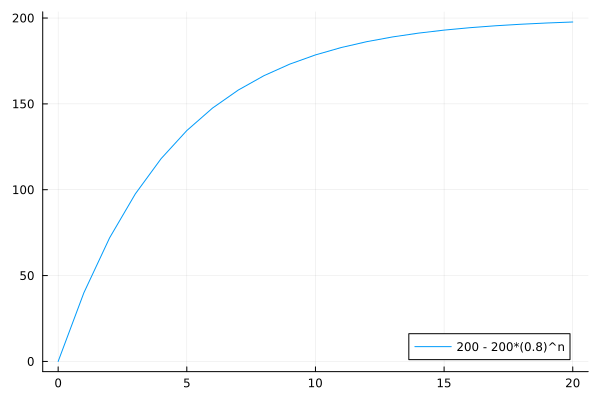
Fig. 11 Plot of a solution to a linear recursion.

As we can see from the horizontal asymptote at 200 in Fig. 11 the solution to our motivating problem: Will there ever be a train long enough to accommodate the 40 people mounting while 20% are dismounting at each station? is to have a train with 200 seats. The plot in Fig. 11 also shows that after 10 stops, the train starts to become very full. While mathematically sound, the solution does not seem realistic enough as the number of people of course has to be a whole number. The Monte Carlo simulation suggested in the exercises can provide a more realistic model.

Exercises

1. Find the z-transform of 1, 2, 3, 1, 2, 3, 1, 2, 3, \(\ldots\)

2. Show that the z-transform of a linear combination of two signals is the linear combination of the two z-transforms of the signals.

3. Set up a Monte Carlo simulation for our motivating problem:

   1. At each stop, each rider on board of the train flips a loaded coin so on average one out of five on board dismount.

   2. Run the simulation for 20 stops, each simulation results in a vector of 20 integers, counting the number of riders on board.

   3. Run the simulation sufficiently many times (e.g.: 1,000) and make a plot of the average counts for each stop. Compare your plot with the plot of the solution of the recursion.

4. Consider the compound interest rate \(i\). \(x(n)\) is the balance after compounding \(n\) times.

   1. Apply the z-transform method to solve

      \[x(n+1) = (1+i) x(n), \quad x_{-1} = 1/(1+i).\]

   2. Use sympy.rsolve to solve the recursion.

5. Compute the partial fraction decomposition of \(\displaystyle \frac{1}{(z-1)(z-2)(z-3)}\).

   You may use computer algebra for this computation.

Bibliography

1. Charles R. MacCluer, start of Chapter 3 of Industrial Mathematics. Modeling in Industry, Science, and Government, Prentice Hall, 2000.

2. J.R. Ragazzini and L.A. Zadeh: The Analysis of Sampled-Data Systems. Transactions of the American Institute of Electrical Engineers, Part II: Applications and Industry. 71 (5): 225-234, 1952.