Filters and Stability

All filters we consider are linear, time invariant, and causal.

Linear, Time Invariant, Causal Filters

Every signal can be written as a linear combinations of sine functions running at increasing frequencies, as \(\sin(2\pi k t)\), \(k=1, 2, \ldots\), see Fig. 12 for the first sine function in this family. Frequencies are measured in Hertz (Hz): \(n\) Hz = \(n\) cycles per second.

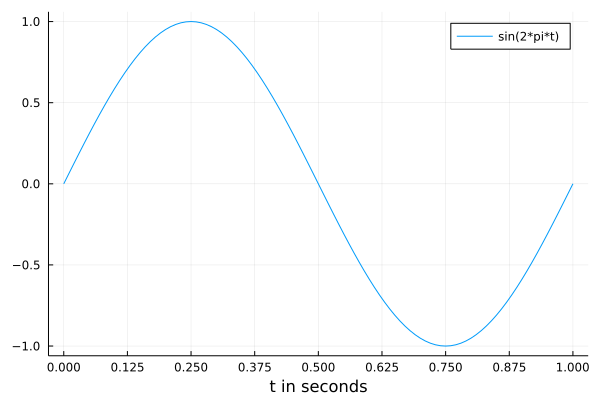
Fig. 12 Sine function running at 1 Hertz, one cycle per second.

Processing a continuous signal happens by taking samples. Sampling at 8 Hertz means taking 8 equidistant samples per second, as illustrated in Fig. 13. Our signal is the represented by \(\{ u_0, u_1, u_2, u_3, u_4, u_5, u_6, u_7, u_0, \ldots \}\), where \(u_k = \sin(2\pi k/8)\), \(k=0,1,2,\ldots,7\).

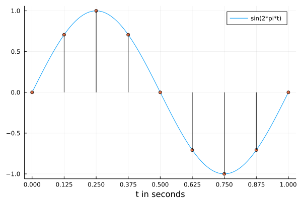
Fig. 13 Sine function running at 1 Hertz, sampled at 8 Hertz.

We can view the unit delay as a filter, as introduced in Fig. 14.

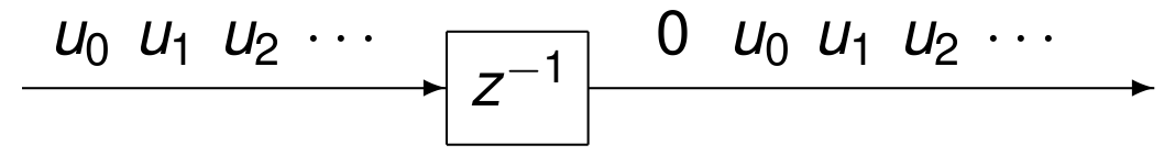
Fig. 14 The unit delay as a filter.

The unit delay has as input \(u = \{ u_0, u_1, u_2, \ldots \}\) has z-transform \(\displaystyle U(z) = \sum_{k=0}^\infty u_k z^{-k}\). The output \(y = \{ 0, u_0, u_1, u_2, \ldots \}\) has z-transform \(Y(z)\), computed below.

\[\begin{split}\begin{array}{rcl} Y(z) & = & {\displaystyle \sum_{k=1}^\infty u_{k-1} z^{-k}} \\ & = & {\displaystyle z^{-1} \sum_{k=1}^\infty u_{k-1} z^{-(k-1)}} ~=~ {\displaystyle z^{-1} \sum_{k=0}^\infty u_k z^{-k}} \\ & = & z^{-1} U(z). \end{array}\end{split}\]

Therefore, the delay of a signal can be viewed as a filter, schematically represented in Fig. 15.

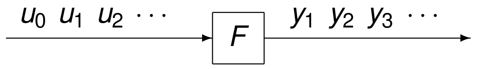
Fig. 15 Schematic representation of a filter.

Definition of a linear, time invariant, causal filter.

A filter \(F\) turns input \(u = \displaystyle \left\{ u_k \vphantom{u^k} \right\}_{k=0}^\infty\) into output \(y = \displaystyle \left\{ y_k \vphantom{y^k} \right\}_{k=0}^\infty\) and is

1. linear: \(F( \alpha u^{(1)} + \beta u^{(2)}) = \alpha F(u^{(1)}) + \beta F(u^{(2)})\),

2. time invariant: \(\displaystyle F\left( \left\{ u_{k+k_0} \vphantom{u^k} \right\}_{k=0}^\infty \right) = \left\{ y_{k + k_0} \vphantom{y^k} \right\}_{k=0}^\infty\), \(k > k_0\), and

3. causal: \(u_k = 0, k < k_0 \Rightarrow y_k = 0, k < k_0\).

For good understanding of this definition, as an exercise, show that the unit delay is a linear, time invariant, and causal filter.

Unit Impulse and Transfer Function

The unit impulse is \(\delta = \{ 1, 0, 0, \ldots \}\). The impulse response is \(h = F \delta = \{ h_0, h_1, h_2, \ldots \}\). Both unit impulse and impulse response are shown in Fig. 16.

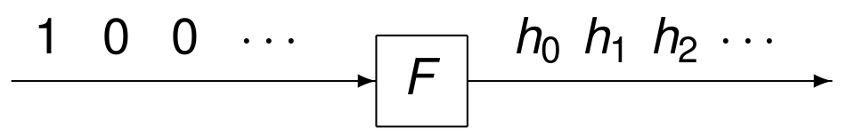
Fig. 16 Schematic representation of the unit impulse and the impulse response.

Theorem charactizing a linear, time invariant, causal filter.

A linear, time invariant, causal filter is entirely determined by the impulse response.

For input \(u\), the \(k\)-th element in the output \(y\) is

\[y_k = u_k h_0 + u_{k-1} h_1 + \cdots + u_1 h_{k-1} + u_0 h_k = \sum_{j=0}^k h_j u_{k-j}.\]

The convolution is denoted by the operator \(\star\), as \(y = h \star u\).

In the frequency domain, the z-transforms of the input and output are

\[U(z) = \sum_{k=0}^\infty u_k z^{-k} \quad \mbox{and} \quad Y(z) = \sum_{k=0}^\infty y_k z^{-k}.\]

The impulse response has as z-transform \(\displaystyle H(z) = \sum_{k=0}^\infty h_k z^{-k}\). The z-transform of \(y = h \star u\) is then

\[Y(z) = H(z) U(z).\]

Definition of the transfer function.

The transfer function of a filter is the z-transform of the impulse response.

Now we can explain the \(z^{-1}\) in the schematic Fig. 14 representing the unit delay as a filter by asking What is the transfer function of the unit delay filter? The transfer function is the z-transform of the impulse response:

• The response of \(\{1, 0, 0, \ldots \}\) is \(\{0, 1, 0, 0, \ldots \}\).

• The z-transform of \(\{0, 1, 0, 0, \ldots \}\) is \(z^{-1}\).

Thus \(z^{-1}\) is the transfer function of the unit delay filter.

Consider computing the output of a filter. Denote

\[\begin{split}\begin{array}{rcl} \delta^{(0)} & = & \{ 1, 0, 0, \ldots \}, \\ \delta^{(1)} & = & \{ 0, 1, 0, \ldots \}, \\ \delta^{(2)} & = & \{ 0, 0, 1, \ldots \}, \quad \mbox{etc.} \end{array}\end{split}\]

then we can write any input \(u\) as \(\displaystyle u = \sum_{k=0}^\infty u_k \delta^{(k)}\).

The output \(y = F u\) can then be written as

\[y = F\left( \sum_{k=0}^\infty u_k \delta^{(k)} \right) = \sum_{k=0}^\infty u_k F \delta^{(k)},\]

because \(F\) is linear.

After decomposing any input \(u\) as linear combinations of properly delayed unit impulses, we construct a formula for the output:

\[\begin{split}\begin{array}{rcl} y & = & u_0 F \delta^{(0)} + u_1 F \delta^{(1)} + u_2 F \delta^{(2)} + \cdots \\ & = & u_0 \{ h_0, h_1, h_2, \ldots \} + u_1 \{ 0, h_0, h_1, h_2, \ldots \} \\ & & +~ u_2 \{ 0, 0, h_0, h_1, h_2, \ldots \} \\ & = & \{ u_0 h_0, u_0 h_1 + u_1 h_0, u_0 h_2 + u_1 h_1 + u_2 h_0, \ldots \} \\ & = & {\displaystyle \sum_{k=0}^\infty ~ \underbrace{\sum_{j=0}^k u_j h_{k-j}}_{y_k}} \end{array}\end{split}\]

The formula for \(y_k\) is a convolution of the input with the impulse response. We proved that the impulse response entirely determines a filter, as stated earlier in the theorem characterizing a linear, time invariant, and causal filter.

Let us now turn to the original function of a filter and removing a signal shown earlier in Fig. 13. Our signal is \(\{ u_0, u_1, u_2, u_3, u_4, u_5, u_6, u_7, u_0, \ldots \}\), where \(u_k = \sin(2\pi k/8)\), \(k=0,1,2,\ldots,7\). Observe, looking at Fig. 13, the symmetry of the samples:

\[u_5 = -u_1, \quad u_6 = -u_2, \quad u_7 = -u_3.\]

Adding a delay will remove the signal. Let the output be defined as follows

\[y_0 = u_0 + u_4, \quad y_1 = u_1 + u_5, \quad y_2 = u_2 + u_6, \quad y_3 = u_3 + u_7.\]

This results in the removal of the signal, as \(y_0 = 0\), \(y_1 = 0\), \(y_2 = 0\), \(y_3 = 0\). The z-transform of \(y\) is \(Y(z)\):

\[Y(z) = U(z) + z^{-4} U(z) = \left( 1 + z^{-4} \right) U(z).\]

The transfer function of the filter is \(H(z) = 1 + z^{-4}\).

Stability

In addition to working with linear, time invariant, and causal filters, we want filters that are stable.

Definition of a stable filter.

A filter is stable if bounded inputs produce bounded outputs.

What are bounded inputs and outputs? Some examples follow.

• \(x = \{ 1, 1, 1, 1, 1, 1, 1, \ldots \}\) is bounded, and so is any constant signal.

• \(x = \{ 1, 2, 4, 8, 16, 32, 64, \ldots \}\) is not bounded.

• \(\displaystyle x = \left\{ 1, \frac{1}{2}, \frac{1}{4}, \frac{1}{8}, \frac{1}{16}, \frac{1}{32}, \frac{1}{64}, \ldots \right\}\) is bounded.

The impulse response determines a linear, time invariant, causal filter.

The transfer function of a stable filter.

Let \(\displaystyle H(z) = \sum_{k=0}^\infty h_k z^{-k}\) be the transfer function of a filter \(F\).

\[F \mbox{ is stable} \quad \Leftrightarrow \quad \sum_{k=0}^\infty |h_k| < \infty.\]

As a corollary, the transfer function \(H(z)\) of a stable filter converges absolutely and uniformly for all \(|z| \geq 1\) to a continuous function.

Amplitude Gain and Phase Shift

The theorem below provides another characterization of a filter.

Theorem on the amplitude and phase shift of a filter.

Let \(\displaystyle H(z) = \sum_{k=0}^\infty h_k z^{-k}\) be the transfer function of a filter \(F\).

For input \(\displaystyle u = \left\{ u_k = \sin(\omega k T) \vphantom{u^k} \right\}_{k=0}^\infty\), \(\displaystyle y = \left\{ y_k = r \sin(\omega k T + \phi) \vphantom{y^k} \right\}_{k=0}^\infty\) is the output, where

• \(r = |H(e^{i \omega T})|\) is the amplitude gain, and

• \(\phi = \mbox{arg} H(e^{i \omega T})\) is the phase shift.

We interpret the input \(u\) as

• \(u = \sin(\omega t)\), \(\omega = 2 \pi n\), at \(n\) Hertz,

• sampled at \(t = kT\), \(T\) is the sampling rate.

Complex numbers appear, the imaginary unit is \(i = \sqrt{-1}\).

The proof of the theorem uses complex numbers. We look at the response of the signal \(s = e^{i \omega T}\).

The input \(\displaystyle u = \left\{ s^k \vphantom{u^k} \right\}_{k=0}^\infty\). Let us compute \(y = h \star u\).

\[y_k = \sum_{j=0}^k h_j u_{k-j} = \sum_{j=0}^k h_j s^{k-j} = s^k \sum_{j=0}^k h_j s^{-j}\]

By the definition of \(H\): \(\displaystyle H(s) = \sum_{j=0}^\infty h_j s^{-j}\). So, we have:

\[y_k = s^k H(s) - s^k \sum_{j=k+1}^\infty h_j s^{-j}.\]

Consider \(k \rightarrow \infty\) and apply the complex exponentiation to the sine function. Our input signal is \(s = e^{i \omega T}\).

\[\begin{split}\begin{array}{cccccr} & s & = & e^{i \omega T} & = & \cos(\omega T) + i \sin(\omega T) \hphantom{\left. \right)} \\ - \left( \right. & s^{-1} & = & e^{-i \omega T} & = & \cos(\omega T) - i \sin(\omega T) \left. \right) \\ \hline & s - s^{-1} & & & = & 2 i \sin(\omega T) \hphantom{\left. \right)} \end{array}\end{split}\]

It then follows:

\[\sin(\omega T) = \frac{1}{2i} \left( s - s^{-1} \vphantom{\frac{1}{2}} \right)\]

and

\[\sin(k \omega T) = \frac{1}{2i} \left( s^k - s^{-k} \vphantom{\frac{1}{2}} \right).\]

We derived \(y_k = s^k H(s)\). Suppose \(H(e^{i \omega T}) = r e^{i \phi}\). What are \(r\) and \(\phi\)?

\[\begin{split}\begin{array}{rcl} { \displaystyle \frac{s^k H(s) - s^{-k} H(s^{-1})}{2 i} } & = & { \displaystyle \frac{1}{2i} \left( \vphantom{\frac{1}{2}} s^k r e^{i \phi} - s^{-k} r e^{-i \phi} \right), \quad s = e^{i \omega T} } \\ & = & { \displaystyle \frac{1}{2i} \left( \vphantom{\frac{1}{2}} e^{k i \omega T + \phi} - e^{-(k i \omega T + \phi)} \right) } \\ & = & r \sin(k \omega T + \phi) \end{array}\end{split}\]

Then indeed, \(r = |H(e^{i \omega T})|\) and \(\phi = \mbox{arg} H(e^{i \omega T})\). The theorem is proven.

Exercises

1. What is the z-transform of a one Hertz sine function sampled at eight Hertz?

2. Show that the unit delay \(F = z^{-1}\) is linear, time invariant, and causal.

3. Noise often happens at high frequency. Give the transfer function of a filter to remove a signal at 60 Hz, sampled at 720 Hz.

   1. Justify the design of your filter.

   2. Which signals are also removed by your filter?

Bibliography

1. Richard C. Dorf and Robert H. Bishop: Modern Control Systems. Nineth Edition, Prentice Hall, 2001.

2. Charles R. MacCluer, middle of Chapter 3 of Industrial Mathematics. Modeling in Industry, Science, and Government, Prentice Hall, 2000.