Bode Plots and Feedback

Bode plots provide an interpretation of the theorem on the amplitude gain and phase shift of a filter.

Bode Plots

We start introducing an averaging filter, shown in Fig. 17.

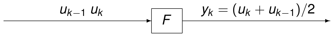
Fig. 17 Schematic of an averaging filter.

For input \(u = \{ u_0, u_1, u_2, \ldots \}\), the output is

\[y = \{ u_0/2, (u_0 + u_1)/2, (u_1 + u_2)/2, \ldots \}.\]

The impulse response, shown in Fig. 18 for the averaging filter, determines a linear, time invariant, causal filter.

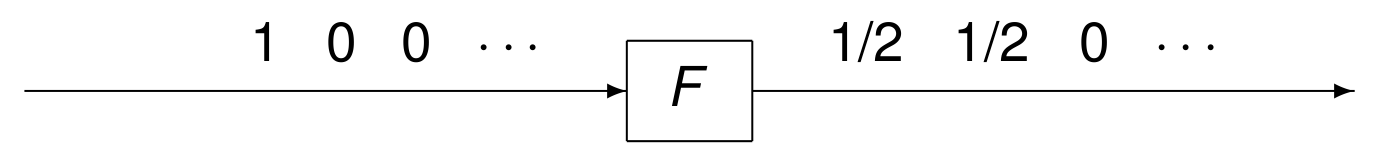
Fig. 18 Schematic of the impulse response of an averaging filter.

The impulse response is finite. The averaging filter is an example of a Finite Impulse Response (FIR) filter.

To determine the transfer function of the averaging filter, denote the z-transform of the input \(u = \{ u_0, u_1, u_2, \ldots \}\) as \(\displaystyle U(z) = \sum_{k=0}^\infty u_k z^{-k}\). The output \(y\) has z-transform

\[Y(z) = (U(z) + z^{-1} U(z))/2 = \left( \frac{1 + z^{-1}}{2} \right) U(z).\]

Therefore, the filter \(F\) has transfer function \(H(z) = (1 + z^{-1})/2\). What is the effect of this filter on signals? To answer this question, consider the theorem on amplitude gain and phase shift, restated below:

Theorem on the amplitude and phase shift of a filter.

Let \(\displaystyle H(z) = \sum_{k=0}^\infty h_k z^{-k}\) be the transfer function of a filter \(F\).

For input \(\displaystyle u = \left\{ u_k = \sin(\omega k T) \vphantom{u^k} \right\}_{k=0}^\infty\), \(\displaystyle y = \left\{ y_k = r \sin(\omega k T + \phi) \vphantom{y^k} \right\}_{k=0}^\infty\) is the output, where

• \(r = |H(e^{i \omega T})|\) is the amplitude gain, and

• \(\phi = \mbox{arg} H(e^{i \omega T})\) is the phase shift.

For the averaging filter \(H(z) = (1+z^{-1})/2\), applying the theorem we compute the amplitude gain \(r\) and phase shift \(\phi\).

For \(u = \sin(\omega t)\), \(\omega = 2 \pi n\), sampled at \(t = k T\):

\[\begin{split}\begin{array}{rcl} H(e^{i \omega T}) & = & (1 + e^{-i \omega T})/2 \\ & = & (1 + \cos(\omega T))/2 - i \sin(\omega T)/2 \end{array}\end{split}\]

For \(x = a + b i\), \(|x| = \sqrt{a^2 + b^2}\) and \(\mbox{arg}(x) = \arctan(b/a)\). The amplitude gain and phase shift are then

\[r = \frac{\sqrt{1 + \cos(\omega T)}}{\sqrt{2}} \quad \mbox{and} \quad \phi = - \arctan \left( \frac{\sin(\omega T)}{1 + \cos(\omega T)} \right).\]

To answer our original question What is the effect of this filter on signals? we need to interpret the formulas, making a plot:

• Fix the sampling rate \(T\) at 1000 samples per second.

• Let the frequencies \(n\) range from 0 to 1000.

To introduce Bode plots, consider the polar plot of the unit circle, which has in polar coordinates a simple representation, shown in Fig. 19.

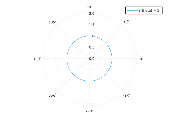
Fig. 19 The unit circle drawn in polar coordinates.

For the averaging filter, we derived the formulas

\[r = \frac{\sqrt{1 + \cos(\omega T)}}{\sqrt{2}} \quad \mbox{and} \quad \phi = - \arctan \left( \frac{\sin(\omega T)}{1 + \cos(\omega T)} \right).\]

and the polar plot is shown in Fig. 20.

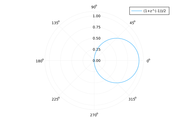
Fig. 20 Polar plot of the amplitude and phase shift of the averaging filter.

In a Bode plot, the amplitude gain and phase shift are separated. The code to produce the Bode plot for the averaging filter in Fig. 21 with Plots.jl is below.

T = 1/1000
freq = 0:1:1000
omega = [2*pi*n for n in freq]
rw = [sqrt(1 + cos(w*T))/sqrt(2) for w in omega]
phi = [-atan(sin(w*T)/(1+cos(w*T))) for w in omega]
gainplot = plot(freq, rw, label="gain")
phaseplot = plot(freq, phi, label ="phase")
plot(gainplot, phaseplot)

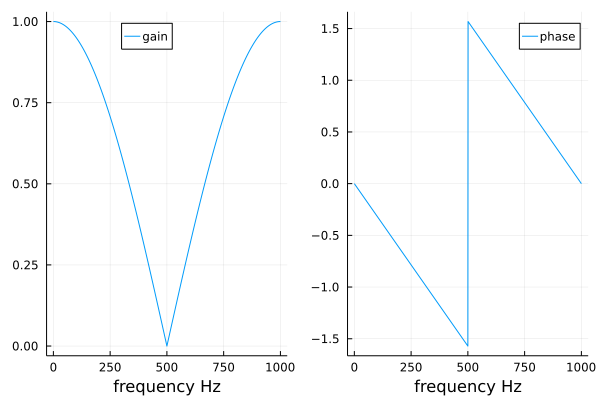
Fig. 21 Bode plot of the averaging filter.

The Bode plot shows the effect of the averaging filter: Higher frequencies are attenuated. This is the lowpass characteristic of this filter: signals running at low frequencies pass.

An exercise asks to remove high frequency noise.

Aliasing and Decibels

Consider:

\[H(e^{i \omega T}) = r e^{i \phi} = H(e^{i(\omega T + 2 \pi)}).\]

The sampled filter response depends only on \(\omega T \mbox{ modulo } 2\pi\).

In western movies, the 24 Hz sampling camera records wagon wheels rotating too slowly or in the retrograde direction. Digital filters cannot distinguish between sampled signals of frequencies congruent modulo the sampling frequency. This phenomenon is aliasing.

Relative power levels are expressed in alert{em decibels} (dB):

\[\frac{p_2}{p_1} \mbox{ dB} = 10 \log_{10} \left( \frac{p_2}{p_1} \right) = 10 \log_{10}(p_2) - 10 \log_{10}(p_1).\]

Why decibels?

1. To comprehend ratios of vastly different magnitudes.

2. The calculations of gains or losses of cascaded systems are transformed to simple additions and subtractions.

Feedback

In Fig. 22 is the schematic of a process \(P\).

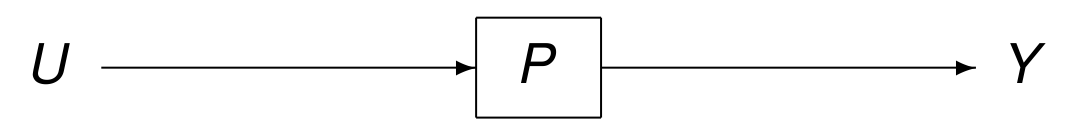
Fig. 22 Schematic of a process.

The transfer function of \(P\) is \(P(z)\), and for z-transforms \(U\) (of the input) and \(Y\) (of the output), we have: \(Y(z) = P(z) U(z)\). The transfer function of the controller or compensator is \(H\), illustrated by Fig. 23. Observe that the input to the controlled process \(P\) is \(U - HY\).

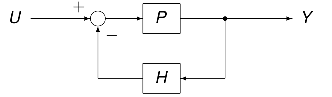
Fig. 23 Schematic of a controlled process.

To compute the transfer function of the controlled process, compute the output of the input \(U - HY\) as follows:

\[\begin{split}\begin{array}{rcl} Y & = & P (U - HY) \\ Y & = & P U - PHY \\ (1+PH) Y & = & P U \end{array}\end{split}\]

Then we obtain

\[Y = \left( \frac{P}{1 + PH} \right) U.\]

as the transfer function of the closed loop system.

The goal of control is to stabilize an unstable plant, illustated by Fig. 24.

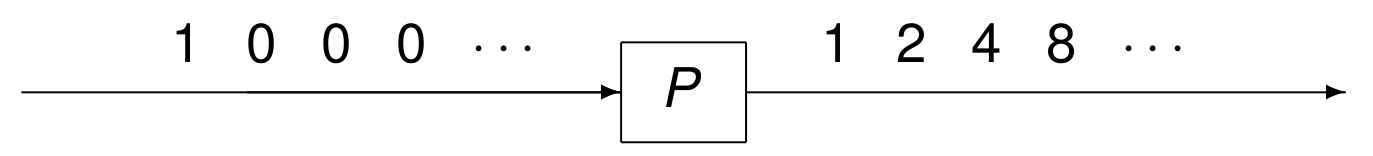
Fig. 24 Schematic of an unstable plant.

The transfer function of \(P\) is

\[P(z) = \frac{z}{z - 2} = \frac{1}{1 - \frac{2}{z}} = 1 + \frac{2}{z} + \frac{4}{z^2} + \frac{8}{z^3} + \cdots + \frac{2^k}{z^k} + \cdots\]

The plant is stabilized by \(H(z) = 3/2\) in the closed loop system shown in Fig. 25.

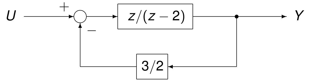
Fig. 25 Schematic of the stabilized plant.

Plant \(P\) and compensator \(H\) have transfer functions

\[P(z) = \frac{z}{z - 2} = \frac{1}{1 - \frac{2}{z}} \quad \mbox{and} \quad H(z) = 3/2.\]

The transfer function of the closed loop is then

\[\begin{split}\begin{array}{rcl} {\displaystyle \frac{P}{1 + PH}} & = & {\displaystyle \frac{1 - \frac{2}{z}}{1 + \frac{3}{2} \left( 1 - \frac{2}{z}\right)}} ~~ = ~~ {\displaystyle \frac{1}{1 + \frac{2}{z} + \frac{3}{2}}} ~~ = ~~ {\displaystyle \frac{1}{\frac{5}{2} - \frac{2}{z}}} \\ & = & {\displaystyle \frac{\frac{2}{5}}{1 - \frac{4}{5} z^{-1}}} \\ & = & {\displaystyle \frac{2}{5} \left( 1 + \frac{4}{5} z^{-1} + \left( \frac{4}{5} \right)^2 z^{-2} + \cdots \right)} \end{array}\end{split}\]

As \(k \rightarrow \infty\), \(\displaystyle \left( \frac{4}{5} \right)^k \rightarrow 0\), so the closed loop system is stable.

Exercises

1. Consider a filter with transfer function

   \[H(z) = \frac{a z + b}{(z - \alpha_1)(z - \alpha_2)}, \quad \alpha_1 \not= \alpha_2.\]

   Show that the filter is stable if and only if \(|\alpha_1| < 1\) and \(|\alpha_2| < 1\).

2. Let \(H(z)\) be the transfer function of a filter to remove a signal at 60 Hz, sampled at 720 Hz.

   1. Make the Bode plot for this filter.

   2. Use the Bode plot to explain which signals are also removed by this filter.

3. Make the Bode plots of the averaging filter for \(T = 1/2000\). Compare the Bode plots for \(T = 1/2000\) and \(T = 1/1000\).

4. Show that an unstable plant with transfer function

   \[P(z) = \frac{1}{1 - \alpha z^{-1}}, \quad |\alpha| > 1,\]

   is stabilized by proportional feedback with transfer function

   \[H(z) = \beta\]

   for any \(\beta > |\alpha| - 1\).

Bibliography

1. Richard C. Dorf and Robert H. Bishop: Modern Control Systems. Nineth Edition, Prentice Hall, 2001.

2. Charles R. MacCluer, end of Chapter 3 of Industrial Mathematics. Modeling in Industry, Science, and Government, Prentice Hall, 2000.