Filter Design

The discrete Fourier transform (DFT) turns a convolution into a componentwise product. The DFT interpolation property is applied to design filters.

Roots of Unity

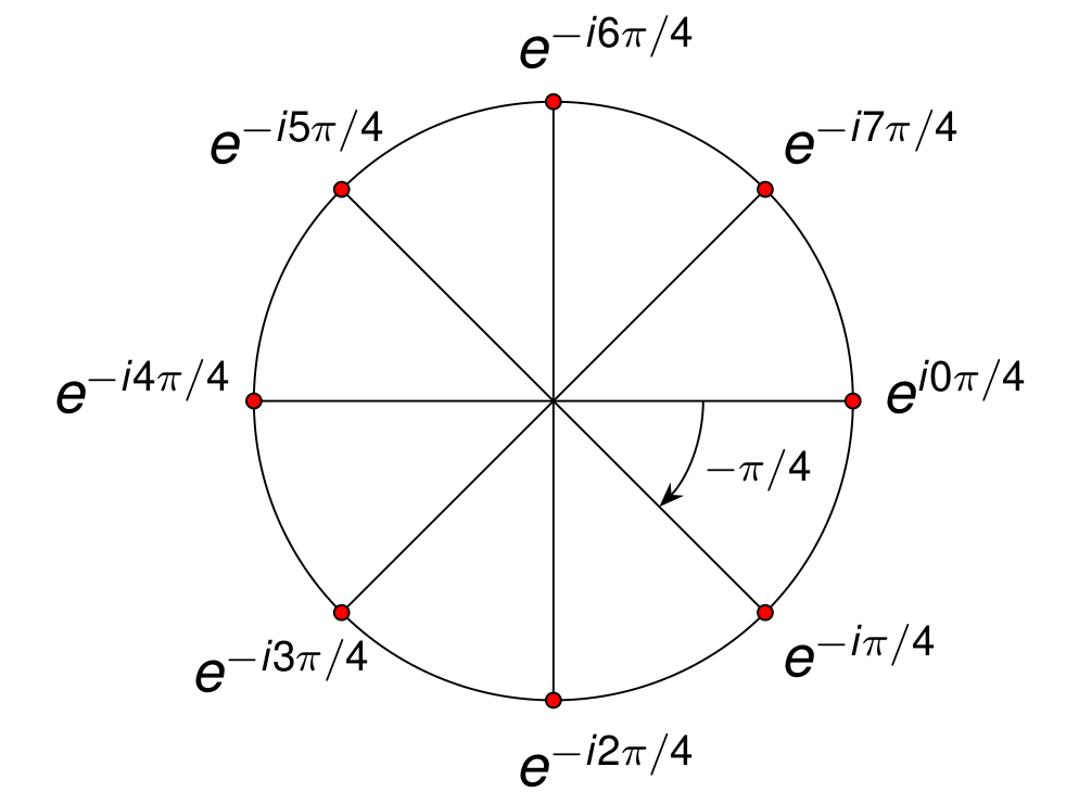
Consider the eight roots of unity, as the eight complex solutions of the equation \(x^8 - 1 = 0\), shown in Fig. 26, in the complex plane. To map the complex numbers into the plane, observe Euler’s formula:

\[\omega = e^{-i \pi/4} = \cos(\pi/4) - i \sin(\pi/4), \quad i = \sqrt{-1}.\]

Fig. 26 The eight roots of unity.

Definition of a root of unity.

The number \(z\) is an n-th root of unity if \(z^n - 1 = 0\).

Definition of a primitive root of unity.

An n-th root of unity is primitive if it is not a k-th root of unity for any \(k < n\).

For \(n > 0\), the n-th primitive root of unity is \(\omega = e^{-i2 \pi/n}\) and \(\omega\) is a root of the equation \(x^n - 1 = 0\), the other \(n-1\) roots are the powers \(\omega^k\), \(k=2,3, \ldots,n\), with \(\omega^n = \omega^0 = 1\).

The root 1 makes the polynomial \(x^n - 1\) factor as follows:

\[\omega^n - 1 = (\omega - 1) \left(1 + \omega + \omega^2 + \cdots + \omega^{n-1} \right) = 0.\]

For \(\omega \not= 1\), we have then

\[1 + \omega + \omega^2 + \cdots + \omega^{n-1} = 0.\]

As the other \(n-2\) roots are powers \(\omega^k\), for \(k=1,2,\ldots,n-1\):

\[1 + \omega^k + \omega^{2k} + \cdots + \omega^{(n-1)k} = 0.\]

For \(k = n\), we have

\[1 + \omega^n + \omega^{2n} + \cdots + \omega^{(n-1)n} = 1 + 1 + 1 + \cdots + 1 = n.\]

We have derived what is known as the Gauss relation, stated formally below.

the Gauss relation.

Let \(\omega\) be a primitive n root of unity and let k be an integer.

\[\begin{split}\sum_{j=0}^{n-1} \omega^{~\!j~\!k} = \left\{ \begin{array}{cl} n & \mbox{if } k/n \mbox{ is an integer}, \\ 0 & \mbox{otherwise.} \end{array} \right.\end{split}\]

Definition of the DFT

Now we are ready to define the discrete Fourier transform (DFT).

Definition of the Discrete Fourier Transform (DFT).

Let \({\bf x} = [x_0, x_1, \ldots, x_{n-1}]^T\) be an n-dimensional vector. The Discrete Fourier Transform of \(\bf x\) is \({\bf y} = [y_0, y_1, \ldots, y_{n-1}]^T\), where

\[y_k = \frac{1}{\sqrt{n}} \sum_{j=0}^{n-1} x_j \omega^{~\!j~\!k}, \quad \omega = e^{-i 2\pi/n}.\]

For example, for \(n=8\), in matrix form the DFT is

\[\begin{split}\left[ \begin{array}{c} y_0 \\ y_1 \\ y_2 \\ y_3 \\ y_4 \\ y_5 \\ y_6 \\ y_7 \end{array} \right] = \frac{1}{\sqrt{n}} \left[ \begin{array}{cccccccc} \omega^{0 \cdot 0} & \omega^{0 \cdot 0} & \omega^{0 \cdot 0} & \omega^{0 \cdot 0} & \omega^{0 \cdot 0} & \omega^{0 \cdot 0} & \omega^{0 \cdot 0} & \omega^{0 \cdot 0} \\ \omega^{1 \cdot 0} & \omega^{1 \cdot 1} & \omega^{1 \cdot 2} & \omega^{1 \cdot 3} & \omega^{1 \cdot 4} & \omega^{1 \cdot 5} & \omega^{1 \cdot 6} & \omega^{1 \cdot 7} \\ \omega^{2 \cdot 0} & \omega^{2 \cdot 1} & \omega^{2 \cdot 2} & \omega^{2 \cdot 3} & \omega^{2 \cdot 4} & \omega^{2 \cdot 5} & \omega^{2 \cdot 6} & \omega^{2 \cdot 7} \\ \omega^{3 \cdot 0} & \omega^{3 \cdot 1} & \omega^{3 \cdot 2} & \omega^{3 \cdot 3} & \omega^{3 \cdot 4} & \omega^{3 \cdot 5} & \omega^{3 \cdot 6} & \omega^{3 \cdot 7} \\ \omega^{4 \cdot 0} & \omega^{4 \cdot 1} & \omega^{4 \cdot 2} & \omega^{4 \cdot 3} & \omega^{4 \cdot 4} & \omega^{4 \cdot 5} & \omega^{4 \cdot 6} & \omega^{4 \cdot 7} \\ \omega^{5 \cdot 0} & \omega^{5 \cdot 1} & \omega^{5 \cdot 2} & \omega^{5 \cdot 3} & \omega^{5 \cdot 4} & \omega^{5 \cdot 5} & \omega^{5 \cdot 6} & \omega^{5 \cdot 7} \\ \omega^{6 \cdot 0} & \omega^{6 \cdot 1} & \omega^{6 \cdot 2} & \omega^{6 \cdot 3} & \omega^{6 \cdot 4} & \omega^{6 \cdot 5} & \omega^{6 \cdot 6} & \omega^{6 \cdot 7} \\ \omega^{7 \cdot 0} & \omega^{7 \cdot 1} & \omega^{7 \cdot 2} & \omega^{7 \cdot 3} & \omega^{7 \cdot 4} & \omega^{7 \cdot 5} & \omega^{7 \cdot 6} & \omega^{7 \cdot 7} \end{array} \right] \left[ \begin{array}{c} x_0 \\ x_1 \\ x_2 \\ x_3 \\ x_4 \\ x_5 \\ x_6 \\ x_7 \end{array} \right]\end{split}\]

The n-by-n matrix in this representation is the Fourier matrix, defined below:

Definition of the Fourier matrix.

For \(\omega = e^{-i 2\pi/n}\), the Fourier matrix is

\[\begin{split}F_n = \frac{1}{\sqrt{n}} \left[ \begin{array}{ccccc} \omega^{0} & \omega^{0} & \omega^{0} & \cdots & \omega^{0} \\ \omega^{0} & \omega^{1} & \omega^{2} & \cdots & \omega^{n-1} \\ \omega^{0} & \omega^{2} & \omega^{4} & \cdots & \omega^{2(n-1)} \\ \vdots & \vdots & \vdots & \ddots & \vdots \\ \omega^{0} & \omega^{n-1} & \omega^{2(n-1)} & \cdots & \omega^{(n-1)^2} \end{array} \right].\end{split}\]

Then for \(\bf x\) and \(\bf y\) two n-dimensional vectors for which

\[{\bf y} = F_n {\bf x},\]

we have that \(\bf y\) is the DFT of \(\bf x\). The Fourier matrix

\[\begin{split}F_n = \frac{1}{\sqrt{n}} \left[ \begin{array}{ccccc} \omega^{0} & \omega^{0} & \omega^{0} & \cdots & \omega^{0} \\ \omega^{0} & \omega^{1} & \omega^{2} & \cdots & \omega^{n-1} \\ \omega^{0} & \omega^{2} & \omega^{4} & \cdots & \omega^{2(n-1)} \\ \vdots & \vdots & \vdots & \ddots & \vdots \\ \omega^{0} & \omega^{n-1} & \omega^{2(n-1)} & \cdots & \omega^{(n-1)^2} \end{array} \right]\end{split}\]

has as inverse (by the Gauss relation):

\[\begin{split}F_n^{-1} = \frac{1}{\sqrt{n}} \left[ \begin{array}{ccccc} \omega^{0} & \omega^{0} & \omega^{0} & \cdots & \omega^{0} \\ \omega^{0} & \omega^{-1} & \omega^{-2} & \cdots & \omega^{-(n-1)} \\ \omega^{0} & \omega^{-2} & \omega^{-4} & \cdots & \omega^{-(2(n-1))} \\ \vdots & \vdots & \vdots & \ddots & \vdots \\ \omega^{0} & \omega^{-(n-1)} & \omega^{-2(n-1)} & \cdots & \omega^{-(n-1)^2} \end{array} \right].\end{split}\]

Observe: \(F_n^{-1} = \overline{F_n}\), the complex conjugate of \(F\). Therefore, this inverse can be used very directly and it defines the inverse discrete Fourier transform, abbreviated by iDFT.

Definition of the inverse discrete Fourier transform (iDFT).

Let \({\bf y} = [y_0, y_1, \ldots, y_{n-1}]^T\) be an n-dimensional vector. The inverse Discrete Fourier Transform of \(\bf y\) is \({\bf x} = [x_0, x_1, \ldots, x_{n-1}]^T\),

\[{\bf x} = F_n^{-1} {\bf y},\]

where \(F_n\) is the n-by-n Fourier matrix.

Componentwise, we have the formulas:

\[x_j = \frac{1}{\sqrt{n}} \sum_{k=0}^{n-1} \left( \omega^{-k} \right)^j y_k, \quad \omega = e^{-i 2\pi/n}, \quad j=0,1,\ldots, n-1.\]

Convolutions and the DFT

The DFT turns convolutions into componentwise products.

In Fig. 27 is the schematic of a filter.

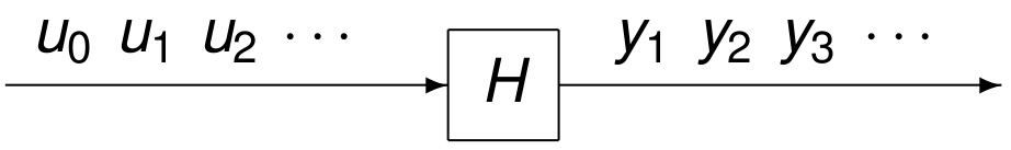
Fig. 27 Schematic of a filter with transfer function \(H\).

A linear, time invariant, causal filter is determined by the impulse response \(\displaystyle \left\{ h_k \vphantom{u^k} \right\}_{k=0}^\infty\) and the transfer function is \(\displaystyle H(z) = \sum_{k=0}^\infty h_k z^{-k}\).

For input \(u\), the k-th element in the output \(y\) is

\[y_k = h_k u_0 + h_{k-1} u_1 + \cdots + h_1 u_{k-1} + h_0 u_k = \sum_{j=0}^k h_{k-j} u_{j}.\]

The convolution is denoted by the operator \(\star\), as \(y = h \star u\).

Consider filtering a periodic signal.

\[u_0, u_1, u_2, u_3, u_0, \ldots \rightarrow (h_0, h_1, h_2, h_3) \rightarrow y_0, y_1, y_2, y_3, y_0, \ldots\]

Let us compute \(y = h \star u\), applying \(\displaystyle y_k = \sum_{j=0}^k h_{k-j} u_{j}\):

\[\begin{array}{rcl} y_0 & = & h_0 u_0 + h_{-1} u_1 + h_{-2} u_2 + h_{-3} u_3. \end{array}\]

By the periodicity: \(h_{-1} = h_3\), \(h_{-2} = h_2\), and \(h_{-3} = h_1\).

\[\begin{split}\begin{array}{rcl} y_0 & = & h_0 u_0 + h_{3} u_1 + h_{2} u_2 + h_{1} u_3 \\ y_1 & = & h_1 u_0 + h_{0} u_1 + h_{3} u_2 + h_{2} u_3 \\ y_2 & = & h_2 u_0 + h_{1} u_1 + h_{0} u_2 + h_{3} u_3 \\ y_3 & = & h_3 u_0 + h_{2} u_1 + h_{1} u_2 + h_{0} u_3 \end{array}\end{split}\]

We start by looking at the discrete Fourier transform of the output. We apply the DFT formula \(\displaystyle y_k = \frac{1}{\sqrt{n}} \sum_{j=0}^{n-1} x_j \omega^{~\!j~\!k}\), for \(n=4\), \(k=1\), on \((y_0, y_1, y_2, y_3)\) as input:

\[\widehat{y}_1 = \frac{1}{\sqrt{4}} \left( y_0 \omega^0 + y_1 \omega^1 + y_2 \omega^2 + y_3 \omega^3 \right).\]

We multiply the formulas with powers of \(\omega\):

\[\begin{split}\begin{array}{rcl} \omega^0 y_0 & = & \omega^0 h_0 u_0 + \omega^0 h_{3} u_1 + \omega^0 h_{2} u_2 + \omega^0 h_{1} u_3 \\ \omega^1 y_1 & = & \omega^1 h_1 u_0 + \omega^1 h_{0} u_1 + \omega^1 h_{3} u_2 + \omega^1 h_{2} u_3 \\ \omega^2 y_2 & = & \omega^2 h_2 u_0 + \omega^2 h_{1} u_1 + \omega^2 h_{0} u_2 + \omega^2 h_{3} u_3 \\ \omega^3 y_3 & = & \omega^3 h_3 u_0 + \omega^3 h_{2} u_1 + \omega^3 h_{1} u_2 + \omega^3 h_{0} u_3 \end{array}\end{split}\]

Adding up the above left hand sides leads to

\[\omega^0 y_0 + \omega^1 y_1 + \omega^2 y_2 + \omega^3 y_3 = 2 \widehat{y}_1.\]

Now we look the right hand sides of

\[\begin{split}\begin{array}{rcl} \omega^0 y_0 & = & \omega^0 h_0 u_0 + \omega^0 h_{3} u_1 + \omega^0 h_{2} u_2 + \omega^0 h_{1} u_3 \\ \omega^1 y_1 & = & \omega^1 h_1 u_0 + \omega^1 h_{0} u_1 + \omega^1 h_{3} u_2 + \omega^1 h_{2} u_3 \\ \omega^2 y_2 & = & \omega^2 h_2 u_0 + \omega^2 h_{1} u_1 + \omega^2 h_{0} u_2 + \omega^2 h_{3} u_3 \\ \omega^3 y_3 & = & \omega^3 h_3 u_0 + \omega^3 h_{2} u_1 + \omega^3 h_{1} u_2 + \omega^3 h_{0} u_3. \end{array}\end{split}\]

Adding up the above right hand sides and collecting terms gives

\[\begin{split}\begin{array}{rcl} & & {\displaystyle u_0 \left( \omega^0 h_0 + \omega^1 h_1 + \omega^2 h_2 + \omega^3 h_3 \right)} \\ & + & {\displaystyle u_1 \left( \omega^0 h_3 + \omega^1 h_0 + \omega^2 h_1 + \omega^3 h_2 \right)} \\ & + & {\displaystyle u_2 \left( \omega^0 h_2 + \omega^1 h_3 + \omega^2 h_0 + \omega^3 h_1 \right)} \\ & + & {\displaystyle u_3 \left( \omega^0 h_1 + \omega^1 h_2 + \omega^2 h_3 + \omega^3 h_0 \right)} \end{array}\end{split}\]

Now we compute the discrete Fourier transform of the coefficients of the transfer function. We apply the DFT formula \(\displaystyle y_k = \frac{1}{\sqrt{n}} \sum_{j=0}^{n-1} x_j \omega^{~\!j~\!k}\), for \(n=4\), \(k=1\), on \((h_0, h_1, h_2, h_3)\) as input:

\[\begin{array}{rcl} \widehat{h}_1 & = & {\displaystyle \frac{1}{\sqrt{4}} \left( h_0 \omega^0 + h_1 \omega^1 + h_2 \omega^2 + h_3 \omega^3 \right).} \end{array}\]

Now we can rewrite the added right hand sides:

\[\begin{split}\begin{array}{rcl} & & {\displaystyle u_0 \left( \omega^0 h_0 + \omega^1 h_1 + \omega^2 h_2 + \omega^3 h_3 \right)} ~~ = ~~ u_0 ~ 2 \widehat{h}_1 \\ & + & {\displaystyle u_1 \left( \omega^0 h_3 + \omega^1 h_0 + \omega^2 h_1 + \omega^3 h_2 \right)} ~~ = ~~ u_1 ~ 2 \widehat{h}_1 ~ \omega^{1} \\ & + & {\displaystyle u_2 \left( \omega^0 h_2 + \omega^1 h_3 + \omega^2 h_0 + \omega^3 h_1 \right)} ~~ = ~~ u_2 ~ 2 \widehat{h}_1 ~ \omega^{2} \\ & + & {\displaystyle u_3 \left( \omega^0 h_1 + \omega^1 h_2 + \omega^2 h_3 + \omega^3 h_0 \right)} ~~ = ~~ u_3 ~ 2 \widehat{h}_1 ~ \omega^{3} \end{array}\end{split}\]

Now, consider the Fourier transform of the input. We apply the DFT formula \(\displaystyle y_k = \frac{1}{\sqrt{n}} \sum_{j=0}^{n-1} x_j \omega^{~\!j~\!k}\), for \(n=4\), \(k=1\), on \((u_0, u_1, u_2, u_3)\) as input:

\[\begin{array}{rcl} \widehat{u}_1 & = & {\displaystyle \frac{1}{\sqrt{4}} \left( u_0 \omega^0 + u_1 \omega^1 + u_2 \omega^2 + u_3 \omega^3 \right).} \end{array}\]

So we found

\[\begin{split}\begin{array}{rcl} 2 \widehat{y}_1 & = & u_0 ~ 2 \widehat{h}_1 + u_1 ~ 2 \widehat{h}_1 ~ \omega^{1} + u_2 ~ 2 \widehat{h}_1 ~ \omega^{2} + u_3 ~ 2 \widehat{h}_1 ~ \omega^{3} \\ & = & {\displaystyle 2 \widehat{h}_1 \left( u_0 + u_1 \omega^{1} + u_2 \omega^{2} + u_3 \omega^{3} \right)} \\ & = & 2 \widehat{h}_1 2 \widehat{u}_1, \end{array}\end{split}\]

or, more in general:

\[\widehat{y}_1 = \sqrt{n} ~ \widehat{h}_1 \widehat{u}_1,\]

where \(\widehat{y} = {\rm DFT}(y)\), \(\widehat{h} = {\rm DFT}(h)\), and \(\widehat{u} = {\rm DFT}(u)\).

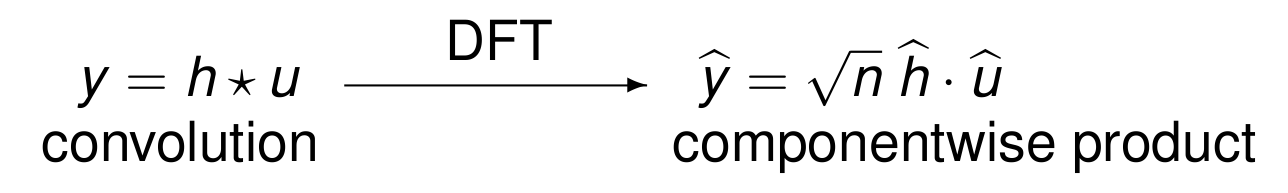
The filter \(H\), schematically shown in Fig. 27, has impulse response \(\displaystyle \left\{ h_k \vphantom{u^k} \right\}_{k=0}^\infty\). The convolution property is shown in Fig. 28.

Fig. 28 The DFT convolution property, where \(\widehat{y} = \mbox{DFT}(y)\), \(\widehat{h} = \mbox{DFT}(h)\), and \(\widehat{u} = {\rm DFT}(u)\).

The calculations done above for \(n=4\) is generalized below.

the DFT convolution property.

The discrete Fourier transform of \(h \star u\) is \(\sqrt{n}\) times the componentwise product of the discrete Fourier transforms of \(h\) and \(u\).

We can formulate the DFT convolution property for any vectors, as done in the theorem below.

the DFT Convolution Property Theorem

Let \(\bf x\) and \(\bf y\) be two n-dimensional vectors. The discrete Fourier transform of \({\bf x} \star {\bf y}\) is \(\sqrt{n}\) times the componentwise product of the discrete Fourier transforms of \(\bf x\) and \(\bf y\).

Then the main statement of this section is DFT convolution theorem.

the DFT Convolution Theorem

Let \(\bf x\) and \(\bf y\) be two n-dimensional vectors. The convolution \({\bf x} \star {\bf y}\) can be computed as

\[{\bf x} \star {\bf y} = \mbox{iDFT} (\sqrt{n}~\mbox{DFT}({\bf x}) \cdot \mbox{DFT}({\bf y})),\]

where \(\mbox{DFT}\) is the discrete Fourier transform, \(\mbox{iDFT}\) is the inverse discrete Fourier transform, and \(\cdot\) is the componentwise product of two vectors.

Interpolation by the DFT

We end this lecture with the statement of the DFT interpolation theorem.

the DFT interpolation theorem.

Consider \(n\) points \(t_j = j/n\), for \(j=0,1,\ldots, n-1\). Let \({\bf x} = [x_0, x_1, \ldots, x_{n-1}]^T\), \({\bf y} = F_n {\bf x}\), where \(F_n\) is the Fourier matrix. Then

\[f(t) = \frac{1}{\sqrt{n}} \sum_{k=0}^{n-1} y_k e^{i 2\pi k t}\]

satisfies \(f(t_j) = x_j\), for \(j=0,1,\ldots,n-1\).

The coefficients \(y_k\) of the discrete Fourier transform are the coefficients of an interpolating function \(f(t)\) in a trigonometric basis.

The proof of the DFT interpolation theorem applies the inverse DFT:

\[{\bf y} = F_n {\bf x}, ~~ f(t) = \frac{1}{\sqrt{n}} \sum_{k=0}^{n-1} y_k e^{i 2\pi k t}, ~~ f(t_j) = x_j, t_j = j/n, ~~ j=0,1,\ldots,n.\]

Proof: we use \({\bf x} = F_n^{-1} {\bf y}\), for \(j=0,1,\ldots,n-1\):

\[\begin{split}\begin{array}{rcl} x_j & = & {\displaystyle \frac{1}{\sqrt{n}} \sum_{k=0}^{n-1} \left( \omega^{-k} \right)^j y_k, \quad \omega = e^{-i2\pi/n}} \\ & = & {\displaystyle \frac{1}{\sqrt{n}} \sum_{k=0}^{n-1} \left( e^{i 2\pi k~\!j/n} \right) y_k} \\ & = & {\displaystyle \frac{1}{\sqrt{n}} \sum_{k=0}^{n-1} \left( e^{i 2\pi k~\!t_j} \right) y_k} ~~= ~~ f(t_j). \end{array}\end{split}\]

The DFT interpolation theorem is applied to design filters, in combination with the theorem on amplitude gain and phase shift, covered in a previous lecture, and restated again below.

Theorem on the amplitude gain and phase shift of filter.

Let \(\displaystyle H(z) = \sum_{k=0}^\infty h_k z^{-k}\) be the transfer function of a filter \(F\). For input \(\displaystyle u = \left\{ u_k = \sin(\omega k T) \vphantom{u^k} \right\}_{k=0}^\infty\), \(\displaystyle y = \left\{ y_k = r \sin(\omega k T + \phi) \vphantom{y^k} \right\}_{k=0}^\infty\) is the output, where (\(\omega = 2\pi n\), \(T\) is the sampling rate),

• \(r = |H(e^{i \omega T})|\) is the amplitude gain, and

• \(\phi = \mbox{\rm arg} H(e^{i \omega T})\) is the phase shift.

The systemematic filter design proceeds in three steps:

1. Make the desired gain \(r = r(t)\) and phase shift \(\phi = \phi(t)\).

2. Evaluate the desired gains and phase shifts at equidistant angles \(\theta_k \in [0, 2\pi]\), \(r_k = r(\theta_k)\), \(\phi_k = \phi(\theta_k)\), \(\widehat{h}_k = r_k e^{i \phi_k}\).

3. \(h = \mbox{iDFT}(\widehat{h})\) is the impulse response, which defines \(H(z)\).

Exercises

1. For \(n=8\), write all n-th roots that are primitive. Verify that for each primitive root \(z\), all other eight roots can be generated by taking powers.

2. Verify the formulas for the inverse of the Fourier transform as follows.

   1. Write a Julia function FourierMatrix with takes on input \(n\) and which returns the Fourier matrix \(F_n\).

   2. Write a Julia function inverseFourierMatrix with takes on input \(n\) and which returns the inverse Fourier matrix \(F_n^{-1}\).

   3. Verify for \(n=8\) that the product of the output of your FourierMatrix with the output of your inverseFourierMatrix is indeed the identity matrix.

3. Verify the DFT convolution property on two random vectors \(\bf x\) and \(\bf y\), for \(n=8\).

   1. Use your FourierMatrix of Exercise 2 to compute the DFT of \(\bf x\) and \(\bf y\), \(\widehat{\bf x} = \mbox{DFT}({\bf x})\) and \(\widehat{\bf y} = \mbox{DFT}({\bf y})\).

   2. Verify that \(\sqrt{8}\) times the componentwise product of \(\widehat{\bf x}\) and \(\widehat{\bf y}\) equals the DFT of \({\bf x} \star {\bf y}\).

4. We derived the statement of the DFT convolution property for \(n=4\) and \(k=1\). Verify the DFT convolution property by symbolic calculation for \(n=4\) and \(k=2\).

5. Verify the DFT interpolation property for \(n = 8\).

   1. Generate a random vector \(\bf x\) of size 8.

   2. Compute \({\bf y} = F_n {\bf x}\), with your FourierMatrix of Exercise 2.

   3. Define the function \(f(t)\).

   4. Verify that \(f(j/n) = x_j\), for \(j=0,1,\ldots,n-1\).

Bibliography

1. Charles R. MacCluer, start of Chapter 4 of Industrial Mathematics. Modeling in Industry, Science, and Government, Prentice Hall, 2000.

2. Timothy Sauer, chapter 10 of Numerical Analysis, second edition, Pearson, 2012.