The Fast Fourier Transform

The fast Fourier transform, abbreviated by FFT, computes the discrete Fourier transform for \(n\) points in time \(O(n \log(n))\).

Time and Frequency Domains

Data is often periodic, e.g.: seasonal temperature fluctuations. To fit periodic data, a basis of cosines and sines works well. The problem we solve is an interpolation problem, stated as follows.

Given \((t_i, f_i)\), \(i=0,1,\ldots,n\), compute the coefficients of

\[y(t) = c_0 + c_1 \cos(2 \pi t) + c_2 \sin(2 \pi t),\]

so \(y(t)\) fits the data \((t_i, f_i)\) best.

A Fourier series approximation is written as

\[y(t) = a_0 + \sum_{k=0}^n \left( a_k \cos(2 \pi k t) + b_k \sin(2 \pi k t) \right).\]

The Fast Fourier Transform solves the interpolation problem in time \(O(n \log(n))\) for \(n\) data points.

There is excellent software available for computing the FFT. Below is a session with Julia which illustrates the transition from the time to the frequency domain.

using Plots
using FFTW

dt = 0.01
t = 0:dt:4
# amplitudes 3 and 5 at frequencies 4 and 2
y = 3*sin.(4*2*pi*t) + 5*sin.(2*2*pi*t)
plot(t, y, yticks=-7:1:7, label="Amplitude in seconds")
F = fft(y)
n = length(y)/2
amps = abs.(F)/n
freq = [0:79]/(2*n*dt)
plot(freq, amps[1:80], xticks=0:1:20,
     label="Frequency (Hz) versus Amplitude")

Observe that the test signal is a linear combination of two sine functions, running at frequencies 4 and 2, and corresponding amplitudes 3 and 5, as can be seen from the definition of \(y(t)\) below:

\[y(t) = 3 \sin(4 \cdot 2 \pi t) + 5 \sin(2 \cdot 2 \pi t).\]

The Julia code makes two plots, shown in Fig. 29 (the plot of \(y(t)\) in the time domain), and in Fig. 30, which shows the essential characterics of the signal in the frequency domain.

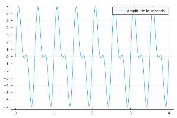
Fig. 29 The plot of \(y(t) = 3 \sin(4 \cdot 2 \pi t) + 5 \sin(2 \cdot 2 \pi t)\).

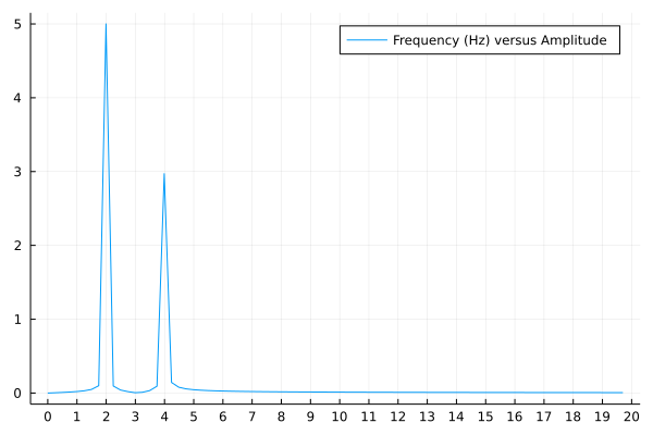
Fig. 30 The plot of the Fourier transform of \(y(t) = 3 \sin(4 \cdot 2 \pi t) + 5 \sin(2 \cdot 2 \pi t)\). Observe the spikes at 2 and 4 (the frequencies) with corresponding heights 3 and 5 (the amplitudes).

The Fast Fourier Transform

For \(n=4\), consider \(\widehat{\bf x} = \frac{1}{\sqrt{4}} M_4 {\bf x}\), with \(\omega = e^{-i 2 \pi/4}\) and

\[\begin{split}M_4 = \left[ \begin{array}{cccc} \omega^0 & \omega^0 & \omega^0 & \omega^0 \\ \omega^0 & \omega^1 & \omega^2 & \omega^3 \\ \omega^0 & \omega^2 & \omega^4 & \omega^6 \\ \omega^0 & \omega^3 & \omega^6 & \omega^9 \end{array} \right] = \left[ \begin{array}{cccc} 1 & 1 & 1 & 1 \\ 1 & \omega & \omega^2 & \omega^3 \\ 1 & \omega^2 & 1 & \omega^2 \\ 1 & \omega^3 & \omega^2 & \omega \end{array} \right]\end{split}\]

In Fig. 31 is the corresponding plot of the four roots of unity.

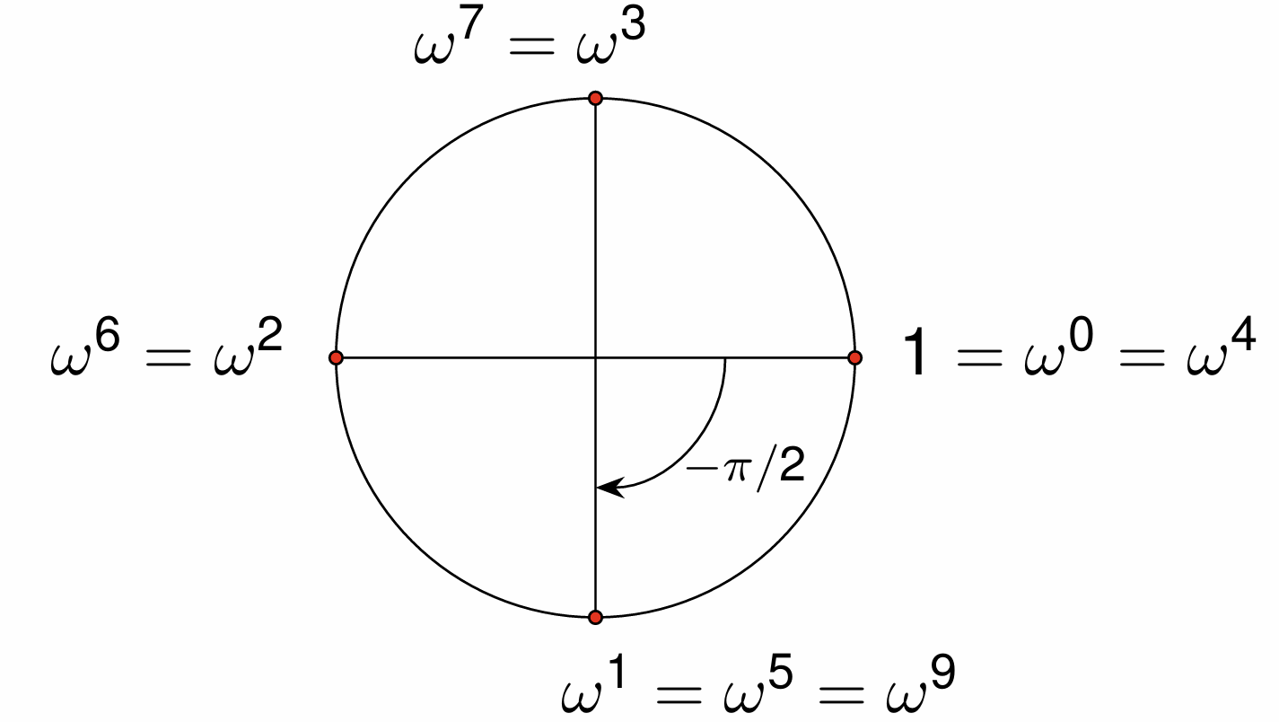
Fig. 31 The four complex roots of unity.

Now we introduce the permute and partition operations on the matrix.

\[\begin{split}M_4 = \left[ \begin{array}{cccc} 1 & 1 & 1 & 1 \\ 1 & \omega & \omega^2 & \omega^3 \\ 1 & \omega^2 & 1 & \omega^2 \\ 1 & \omega^3 & \omega^2 & \omega \end{array} \right] \quad P = \left[ \begin{array}{cccc} 1 & 0 & 0 & 0 \\ 0 & 0 & 1 & 0 \\ 0 & 1 & 0 & 0 \\ 0 & 0 & 0 & 1 \\ \end{array} \right]\end{split}\]

Multiplying \(M_4\) with \(P\) swaps columns 2 and 3.

\[\begin{split}M_4 P = \left[ \begin{array}{cccc} 1 & 1 & 1 & 1 \\ 1 & \omega^2 & \omega & \omega^3 \\ 1 & 1 & \omega^2 & \omega^2 \\ 1 & \omega^2 & \omega^3 & \omega \end{array} \right] = \left[ \begin{array}{cc|cc} 1 & 1 & 1 & 1 \\ 1 & \omega^2 & \omega & \omega^3 \\ \hline 1 & 1 & \omega^2 & \omega^2 \\ 1 & \omega^2 & \omega^3 & \omega \end{array} \right]\end{split}\]

Observe the repeated occurrence of \(M_2\):

\[\begin{split}M_2 = \left[ \begin{array}{cc} 1 & 1 \\ 1 & \omega^2 \end{array} \right], \quad F_2 = \frac{1}{\sqrt{2}} M_2.\end{split}\]

The matrix \(D_2\) is obtained via a multiplication with \(\omega\).

\[\begin{split}M_4 P = \left[ \begin{array}{cc|cc} 1 & 1 & 1 & 1 \\ 1 & \omega^2 & \omega & \omega^3 \\ \hline 1 & 1 & \omega^2 & \omega^2 \\ 1 & \omega^2 & \omega^3 & \omega \end{array} \right], \quad M_2 = \left[ \begin{array}{cc} 1 & 1 \\ 1 & \omega^2 \end{array} \right], \quad F_2 = \frac{1}{\sqrt{2}} M_2.\end{split}\]

Multiplying the second row by \(\omega\) of \(M_2\), via a matrix multiplication:

\[\begin{split}\left[ \begin{array}{cc} 1 & 0 \\ 0 & \omega \end{array} \right] \left[ \begin{array}{cc} 1 & 1 \\ 1 & \omega^2 \end{array} \right] = \left[ \begin{array}{cc} 1 & 1 \\ \omega & \omega^3 \end{array} \right] = D_2 M_2,\end{split}\]

where \(D_2\) is the multiplier matrix:

\[\begin{split}D_2 = \left[ \begin{array}{cc} 1 & 0 \\ 0 & \omega \end{array} \right].\end{split}\]

Consider flipping signs:

\[\begin{split}M_4 P = \left[ \begin{array}{cc|cc} 1 & 1 & 1 & 1 \\ 1 & \omega^2 & \omega & \omega^3 \\ \hline 1 & 1 & \omega^2 & \omega^2 \\ 1 & \omega^2 & \omega^3 & \omega \end{array} \right], \quad M_2 = \left[ \begin{array}{cc} 1 & 1 \\ 1 & \omega^2 \end{array} \right], \quad D_2 = \left[ \begin{array}{cc} 1 & 0 \\ 0 & \omega \end{array} \right].\end{split}\]

and we have

\[\begin{split}\left[ \begin{array}{cc} \omega^2 & \omega^2 \\ \omega^3 & \omega \end{array} \right] = \left[ \begin{array}{cc} -1 & -1 \\ -\omega & -\omega^3 \end{array} \right] = - D_2 M_2.\end{split}\]

The butterfly matrix is illustrated in Fig. 32.

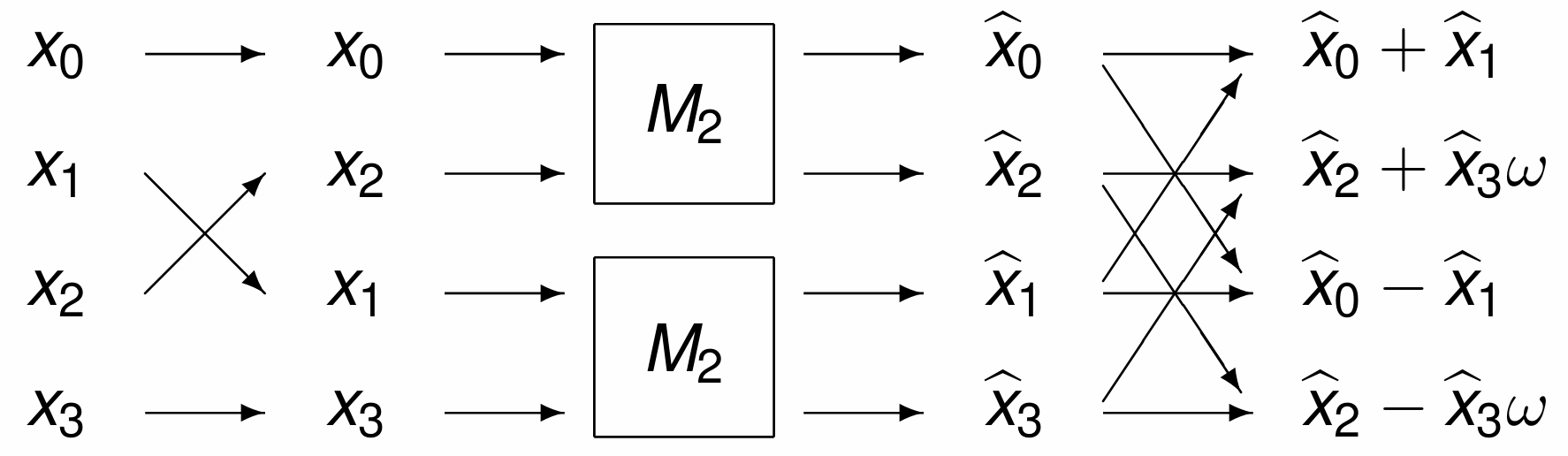
Fig. 32 The 2-dimensional butterfly matrix.

\[\begin{split}M_2 = \left[ \begin{array}{cc} 1 & 1 \\ 1 & \omega^2 \end{array} \right] \quad \mbox{and} \quad D_2 = \left[ \begin{array}{cc} 1 & 0 \\ 0 & \omega \end{array} \right]\end{split}\]

we rewrite \(M_4 P\) as

\[\begin{split}\left[ \begin{array}{cc|cc} 1 & 1 & 1 & 1 \\ 1 & \omega^2 & \omega & \omega^3 \\ \hline 1 & 1 & \omega^2 & \omega^2 \\ 1 & \omega^2 & \omega^3 & \omega \end{array} \right] = \left[ \begin{array}{rr} M_2 & D_2 M_2 \\ M_2 & -D_2 M_2 \end{array} \right] = \left[ \begin{array}{rr} I_2 & D_2 \\ I_2 & -D_2 \end{array} \right] \left[ \begin{array}{cc} M_2 & 0 \\ 0 & M_2 \end{array} \right].\end{split}\]

The matrix

\[\begin{split}B_4 = \left[ \begin{array}{rr} I_2 & D_2 \\ I_2 & -D_2 \end{array} \right], \quad I_2 = \left[ \begin{array}{rr} 1 & 0 \\ 0 & 1 \end{array} \right],\end{split}\]

is called the butterfly matrix. For \(n=4\), the effect of the butterfly matrix \(B_4\) is shown below:

\[\begin{split}B_4 \left[ \begin{array}{c} \widehat{x_0} \\ \widehat{x_2} \\ \widehat{x_1} \\ \widehat{x_3} \end{array} \right] = \left[ \begin{array}{rrrr} 1 & 0 & 1 & 0 \\ 0 & 1 & 0 & \omega \\ 1 & 0 & -1 & 0 \\ 0 & 1 & 0 & -\omega \end{array} \right] \left[ \begin{array}{c} \widehat{x_0} \\ \widehat{x_2} \\ \widehat{x_1} \\ \widehat{x_3} \end{array} \right] = \left[ \begin{array}{l} \widehat{x_0} + \widehat{x_1} \\ \widehat{x_2} + \widehat{x_3} \omega \\ \widehat{x_0} - \widehat{x_1} \\ \widehat{x_2} - \widehat{x_3} \omega \end{array} \right].\end{split}\]

For any \(n\), we apply the recursive factorization

\[\begin{split}M_n = B_n \left[ \begin{array}{cc} M_{n/2} & 0 \\ 0 & M_{n/2} \end{array} \right] P_n\end{split}\]

where the partition \(P_n\) reorders the even and odd indexed numbers, with the butterfly matrix

\[\begin{split}B_n = \left[ \begin{array}{rr} I_{n/2} & D_{n/2} \\ I_{n/2} & - D_{n/2} \end{array} \right],\end{split}\]

where \(I_{n/2}\) is the identity matrix of dimension \(n/2\), and \(D_{n/2}\) is the diagonal matrix with on its diagonal

\[1, \omega, \omega^{2}, \ldots, \omega^{n/2-1}.\]

To the recurrence \(T(n) \leq 2 T(n/2) + O(n)\), we apply the following theorem:

Theorem on resolving an n*log(n) recurrence.

If \(T(n) \leq 2 T(n/2) + c_1 n\) and \(T(2) \leq c_2\), for positive constants \(c_1\) and \(c_2\), then \(T(n)\) is \(O(n \log(n))\).

Theorem on the cost of FFT.

On vectors of size \(n\), the FFT runs in \(O(n \log(n))\) time.

For the inverse FFT, \(F^{-1}_n = \overline{F}_n\), so

\[F^{-1}_n y = \overline{F}_n y = \overline{F_n \overline{y}},\]

and no extra work is needed.

Filter Design

To design filters, we apply the convolution property of the discrete Fourier transform, shown as a diagram in Fig. 33. The inverse discrete Fourier transform (iDFT) applied to the componentwise product \(\widehat{x} \bullet \widehat{y}\) of the discrete Fourier transforms (DFTs) \(\widehat{x}$ and $\widehat{y}\), respectively of \(x\) and \(y\), equals the convolution \(x \star y\).

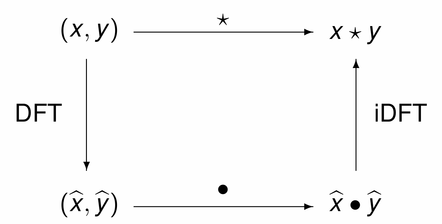
Fig. 33 The convolution property of the discrete Fourier transform.

As the fast Fourier fourier transform of vectors of size \(n\) can be computed in time \(O(n \log(n))\), the \(O(n^2)\) cost of a convolution is reduced to time \(O(n \log(n))\), as illustrated in Fig. 34.

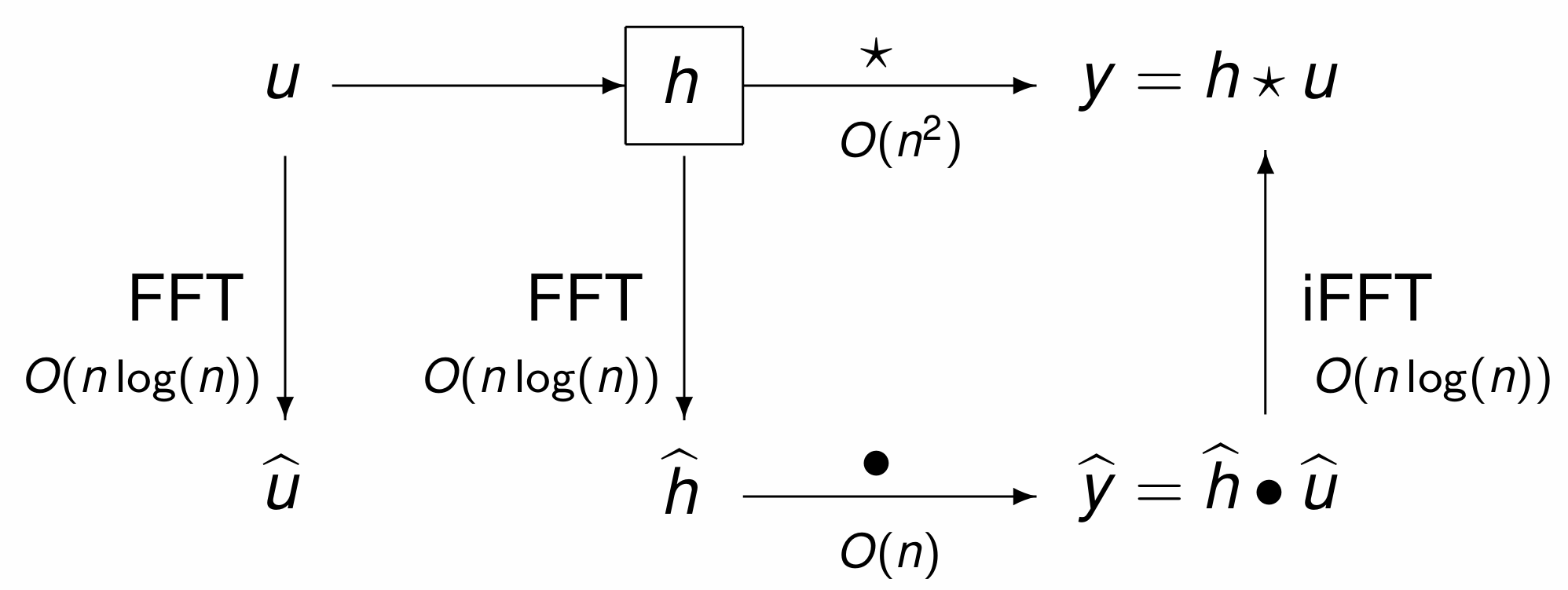
Fig. 34 The FFT reduces the cost of a convolution to \(O(n \log(n))\).

Exercises

1. Use your FourierMatrix of Exercise 2 of the previous lecture, section 4.1, to compare the outcome of \(F_n {\bf x}\) computed with the \(F_n\) computed with your FourierMatrix and the output of FFTW.fft.

   • Do the comparison on a random vector \(\bf x\) of size \(n = 8\).

   • Does the FFTW.fft use the normalization factor \(1/\sqrt{n}\)?

2. Write a Julia function ButterflyMatrix which takes on input the dimension \(n\) and which returns the butterfly matrix of dimension \(n\).

   To verify the decomposition, define a function mFourierMatrix that takes on input the dimension \(n\) and which returns the Fourier matrix times \(\sqrt{n}\).

   For \(n=8\), verify the relationship between mFourierMatrix (n) and ButterflyMatrix (n).

3. Generate random vectors for size \(2^k\), for \(k=10, 11, \ldots, 20\).

   • For each random vector, record the time for FFTW.fft.

   • Do you observe the \(O(n \log(n))\) time?

Bibliography

1. Matteo Frigo and Steven G. Johnson: The Design and Implementation of FFTW3. Proc. IEEE 93(2): 216–231, 2005.

2. Charles R. MacCluer, Chapter 4 of Industrial Mathematics. Modeling in Industry, Science, and Government, Prentice Hall, 2000.

3. Timothy Sauer, chapter 10 of Numerical Analysis, second edition, Pearson, 2012.