Applications of the FFT
In this third lecture in the fourth week, we consider applications of the FFT.
Spectral Analysis
The \(O(n \log(n))\) time of the Fast Fourier Transform allows for the online filtering of data. We distinguish between three types of filters:
lowpass: only low frequencies pass,
highpass: only high frequencies pass, and
bandpass: only frequencies within a band do pass.
Filtering with the FFT proceeds in three steps:
transform the input data to the frequency domain,
remove the components of unwanted frequencies, and
transform the filtered data to the time domain.
Consider again our test signal of the previous lecture:
The code block below adds low applitude noise, plots the signal in the time domain, in Fig. 35.
using Plots
using FFTW

dt = 0.01
t = 0:dt:4
y = 3*sin.(4*2*pi*t) + 5*sin.(2*2*pi*t)
ynoise = y + 0.3*randn(length(y))
dt = 0.01
t = 0:dt:4
y = 3*sin.(4*2*pi*t) + 5*sin.(2*2*pi*t)
plot(t, y, yticks=-7:1:7, label="signal"
     xlabel="Time in Seconds", ylabel="Amplitude")
plot!(t, ynoise, color="red", label="noisy signal")
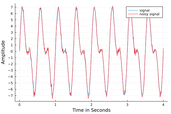
Fig. 35 A noisy signal in the time domain.
The FFT transform computes the spectrum, shown in Fig. 36. Observe: the spectrum of the noisy signal has the same two spikes at the two frequencies and their corresponding amplitudes.
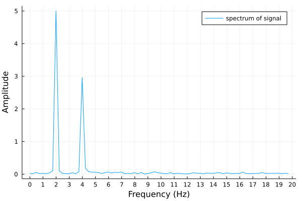
Fig. 36 Spectrum of a noisy signal in the frequency domain.
Observing the spectrum of the noisy signal, we see that the noisy appears for all frequencies, but at low amplitude. Then the code to remove the low amplitude noise is simple:
filteredF = [x*Int(abs(x) > 50) for x in F];
All numbers in magnitude less than 50 are replaced by zero.
The semicolon ; suppresses the output.
Finding the good threshold requires inspecting the numbers.
The filtered spectrum is shown in Fig. 37.
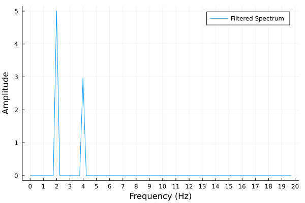
Fig. 37 The filtered spectrum of a noisy signal.
To reconstruct the signal, we apply the inverse FFT.
yfiltered = ifft(filteredF)
To plot the filtered signal,
we plot only the real part of the output of the ifft,
with the code below:
plot(t, real(yfiltered),
     yticks=-7:1:7,
     label="filtered signal",
     xlabel="Time in Seconds",
     ylabel="Amplitude")
The filtered signal is shown in Fig. 38.
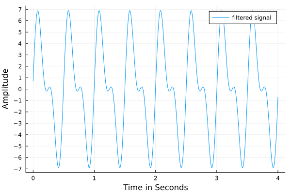
Fig. 38 The filtered signal, after removing the low amplitude noise.
With the FFT and iFFT we can remove unwanted frequencies: in the spectrum, set the amplitudes for the unwanted frequencies to zero.
Image Processing
To introduce our second application of the FFT, consider a familiar image in Fig. 39.
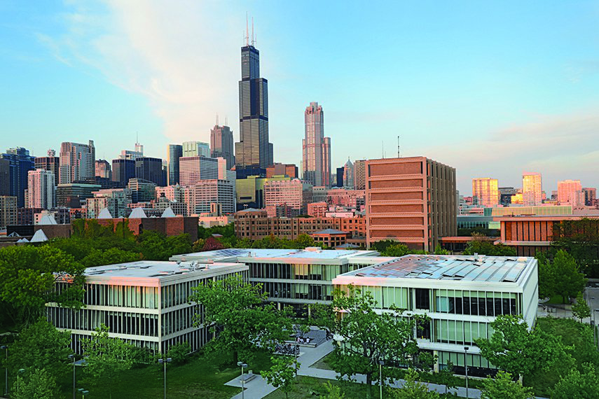
Fig. 39 A familiar image as test for image processing.
Images are matrices of RGB codes. If the image in Fig. 39
is saved in the file buildingsky.png, then loading the image into a
Julia session happens as follows:
using Images
A = load("buildingsky.png")
size(A)
The load displays the image.
The output of size(A) is \((570, 855)\),
as A has 570 rows and 855 columns.

Fig. 40 A selection of the middle of our test image.
Selecting the middle of the image, shown in Fig. 40 is done by the commands below:
m1 = Int(size(A,1)/2)
m2 = Int(round(size(A,2)/2))
Amiddle = A[m1-20:m1+20,m2-20:m2+20]
The matrix representing the images stores the red, green, blue intensities for each pixel. Let us look at one element of the matrix. The commands
a = A[1,1]; typeof(a)
returns RGB{N0f8}.
The RGB is the type of the Red, Green, Blue intensities.
The output of dump(a) is
RGB{N0f8}
  r: N0f8
    i: UInt8 0x81
  g: N0f8
    i: UInt8 0xd3
  b: N0f8
    i: UInt8 0xfb
The components of a are a.r, a.g, and a.b,
represented as 8-bit unsigned integers.
Convert components to floats, and we can compute with the intensities,
as done below:
agray = RGB{Float32}((Float32(a.r)
                    + Float32(a.g)
                    + Float32(a.b))/3)
Averaging the intensities lead to a grayscale picture, shown in Fig. 41.
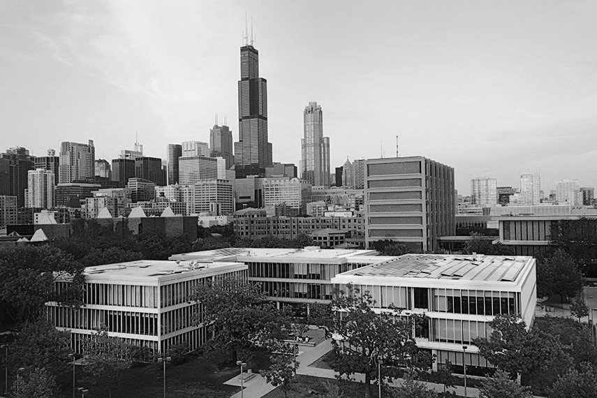
Fig. 41 The grayscale version of our test image.
The complete code to convert an image to grayscale is below:
Agray = zeros(size(A,1), size(A,2))
Agray = Matrix{RGB{Float32}}(Agray)
for i=1:size(A,1)
    for j=1:size(A,2)
        a = A[i,j]
        b = RGB{Float32}((Float32(a.r)
                        + Float32(a.g)
                        + Float32(a.b))/3)
        Agray[i,j] = b
    end
end
In the grayscale image, all intensities are the same. The matrix of RGB codes can then be converted into a matrix of floats as done below:
C = zeros(size(Agray,1), size(Agray,2))
for i=1:size(Agray,1)
    for j=1:size(Agray,2)
        C[i,j] = Agray[i,j].r
    end
end
The grayscale matrix is used for the remaining computations. If we want to work with colors, then we can work with three different matrices, one matrix of each intensity.
One application is the blurring and deblurring of images for safe transmission. Let \(X\) be an m-by-n matrix, representing an image.
\(B\) is a blur matrix.
Compute \(Y = B \star X\) to blur the image stored in \(X\), the \(\star\) is the matrix-matrix multiplication. Because of the blurring, \(Y\) is safe for transmission.
To deblur the image, do \(X = B^{-1} \star Y\).
Two computational problems:
The matrix-matrix multiplication \(\star\) costs \(O(n^3)\).
Computing the inverse \(B^{-1}\) also costs \(O(m^3)\).
To allieviate those computational problems, we will appy two dimensional Fourier transforms.
For \(X\), as an m-by-n matrix, consider
Let \(\omega_m\) be the m-th primitive root: \(\omega_m^m - 1 = 0\).
Let \(\omega_n\) be the n-th primitive root: \(\omega_n^n - 1 = 0\).
Then the discrete Fourier transform of \(X\) is \(\widehat{X}\) with entries
The rowwise and columnwise formulas are the same because of the distributive properties of addition with multiplication. In Fig. 42 is the schematic summary of the application of the FFT to blur and deblur images. Matrix-matrix multiplications and inverse computations are avoided:
The \(\bullet\) is the componentwise multiplication, and
the \(/\) is the componentwise division.
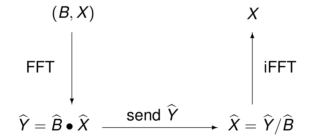
Fig. 42 Schematic of the application of the FFT to blur images.
The plain code to blur an image with matrix-matrix multiplication is below:
B = randn(size(C,1), size(C,1))
Y = B*C
D = zeros(size(Y,1), size(Y,2))
D = Matrix{RGB{Float32}}(D)
for i=1:size(Y,1)
    for j=1:size(Y,2)
        a = Y[i,j]
        if a < 0
            a = 0.0
        end
        if a > 1
            a = 1.0
        end
        D[i,j]= RGB{Float32}(a,a,a)
    end
end
The blurred grayscale picture is shown in Fig. 43.

Fig. 43 The blurred grayscale image of our test picture.
Now the code for the application of the FFT is developed. For the componentwise multiplication \(\widehat{Y} = \widehat{B} \bullet \widehat{X}\), the matrix \(B\) needs to be of the same size as \(X\). Therefore, We extend \(B\) with ones on the diagonal and zeros off the diagonal:
BB = zeros(size(C,2), size(C,2))
BB[1:size(B,1),1:size(B,2)] = B
for i in size(B,1)+1:size(BB,1)
    BB[i,i] = 1.0
end
The code for the blurring with FFT and componentwise products is below:
using FFTW

fftB = fft(BB)
fftC = fft(C)
fftY = zeros(size(C,1), size(C,2))
fftY = Matrix{Complex{Float64}}(fftY)
for i=1:size(C,1)
    for j=1:size(C,2)
        fftY[i,j] = fftB[i,j]*fftC[i,j]
    end
end
The fftY holds the blurred image, safe for transmission.
The received data is fftY.
To compute the original image, we first do
\(\widehat{X} = \widehat{Y}/\widehat{B}\), as below:
fftX = zeros(size(C,1), size(C,2))
fftX = Matrix{Complex{Float64}}(fftY)
for i=1:size(C,1)
    for j=1:size(C,2)
        fftX[i,j] = fftY[i,j]/fftB[i,j]
    end
end
And then apply the inverse FFT:
X = ifft(fftX)
deblurred = zeros(size(X,1), size(X,2))
deblurred = Matrix{RGB{Float32}}(deblurred)
for i=1:size(X,1)
    for j=1:size(X,2)
        x = Float32(real(X[i,j]))
        deblurred[i,j] = RGB{Float32}(x,x,x)
    end
end
The deblurred matrix contains the representation
of the original grayscale image in Fig. 41.
Exercises
Make a signal with three components:
the first sine has amplitude 5 and runs at 2Hz,
the second sine has amplitude 3 and runs at 8Hz, and
the third sine has amplitude 1 and runs at 16Hz.
Use this signal to demonstrate the application of the FFT for three types of filters:
Low pass: remove all frequencies higher than 6Hz.
High pass: remove all frequencies lower than 10Hz.
Make a signal with three components:
the first sine has amplitude 5 and runs at 2Hz,
the second sine has amplitude 3 and runs at 8Hz, and
the third sine has amplitude 1 and runs at 16Hz.
Use this signal to demonstrate the application of the FFT to
double the amplitude for frequencies ranging from 6Hz to 10Hz,
multiply the amplitudes for all other frequencies by 0.1.
Take an image, for example our familiar picture in Fig. 39 and give the operations to increase the green intensities by 10%.
In processing medical images, the images are of round objects, e.g.: brain scans produced by Magnetic Resonance Imaging (MRI). Search the literature for methods on the applications of the FFT on data that is not scanned on a grid that is not rectangular, but polar.
Bibliography
Charles R. MacCluer, end of Chapter 4 of Industrial Mathematics. Modeling in Industry, Science, and Government, Prentice Hall, 2000.
Timothy Sauer, chapter 10 of Numerical Analysis, second edition, Pearson, 2012.
Summary of the Last Six Lectures
In the past six lectures, we provided a computational overview of signal processing and filter design.
The z-transform of a sequence shows the grow or decay factors.
Linear, time invariant, and causal filters are determined entirely by the impulse response, or the coefficients of its transfer function.
Bode plots show the amplitude gain and phase shift of the evaluated transfer function.
The Discrete Fourier Transform (DFT) turns convolutions into componentwise products.
The Fast Fourier Transform (FFT) executes the DFT in \(O(n \log(n))\) time.
Applications of the FFT include the removal of low amplitude noise; lowpass, highpass, bandpass filters; and image blurring.