Linear Programming

After the first week of project presentations, we start the sixth week looking at mathematical optimization.

Optimization Problems

A linear programming problem is particular form of a mathematical optimization problem, motivated by production planning. We want to maximize profit and minimize cost, expressed as

\[\begin{split}\begin{array}{lcl} \mbox{maximize profit} & & \mbox{minimize cost} \\ \mbox{subject to} & & \mbox{subject to} \\ \hspace{5mm} \mathrm{E}({\bf x}) = {\bf a} & equalities & \hspace{5mm} \mathrm{E}({\bf x}) = {\bf a} \\ \hspace{5mm} \mathrm{I}({\bf x}) \leq {\bf b} & inequalities & \hspace{5mm} \mathrm{I}({\bf x}) \geq {\bf b} \end{array}\end{split}\]

Definition of a linear programming problem.

A linear programming problem is an optimization problem

• with one linear objective functions; and

• all constraints (equalities and inequalities) are linear.

LP program is short for Linear Programming problem. Viewing linear programming geometrically, the linear constraints define a polyhedron, illustrated by Fig. 44.

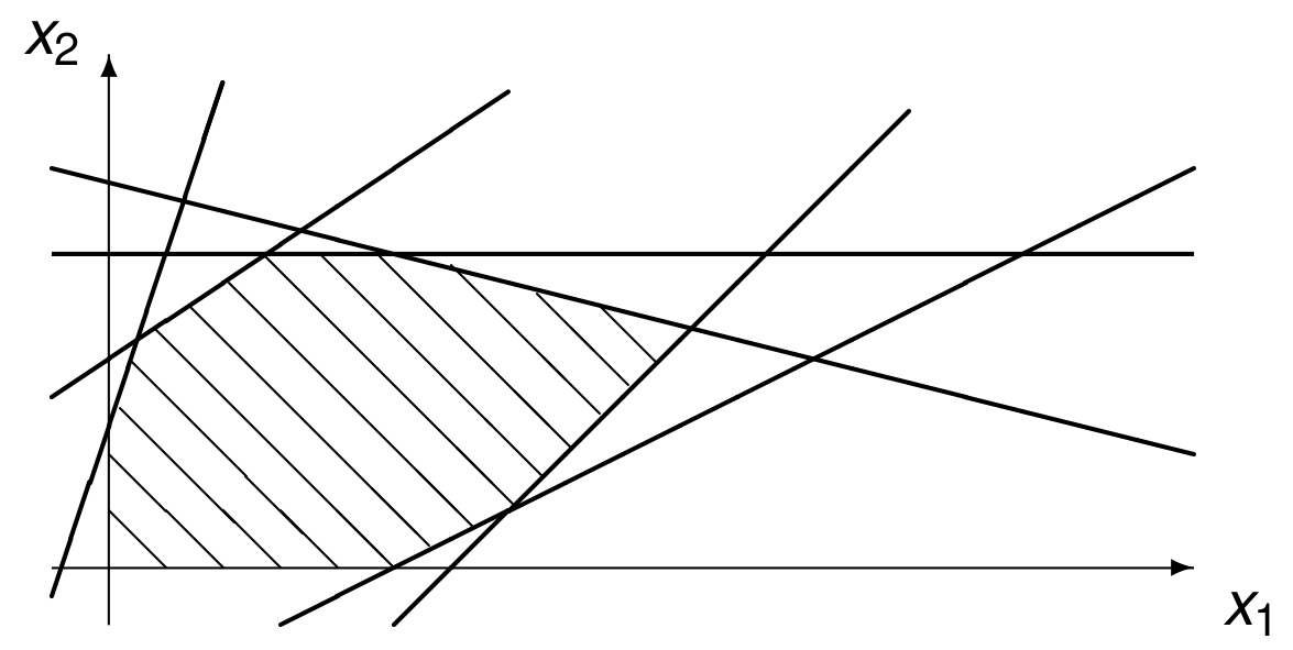
Fig. 44 A polyhedron as the intersection of half planes.

We want the optimization problem to be feasible and well posed defined below:

1. If the polyhedron is not empty, then the problem is feasible.

2. If the polyhedron is bounded, then the problem is well posed.

An LP problem can have infinitely many solutions. Looking at Fig. 44 observe that, if we consider any two points in the polyhedron, then any point on the line segment connecting those two points also belongs to the polyhedron. A polyhedron is convex.

Definition of convex combination.

For points \(\bf x\) and \(\bf y\), a convex combination of \(\bf x\) and \(\bf y\) is

\[\lambda {\bf x} + (1-\lambda) {\bf y}, \mbox{ for } \lambda \in [0,1].\]

If \(\bf x\) and \(\bf y\) are solutions to an LP problem, then any convex combination of \(\bf x\) and \(\bf y\) is also a solution.

Consider the standard form for a linear minimization problem:

\[\begin{split}\begin{array}{lcl} {\rm min}~ {\bf c}^T {\bf x} & & {\bf c}, {\bf x} \in {\mathbb R}^n, \\ {\rm subject~to}~ A {\bf x} \geq {\bf b} & & A \in {\mathbb R}^{m \times n}, {\bf b} \in {\mathbb R}^m. \end{array}\end{split}\]

To turn the inequalities into equalities, we add slack variables \({\bf z} \in {\mathbb R}^m\):

\[A {\bf x} \geq {\bf b} \quad {\rm becomes} \quad A {\bf x} - {\bf z} = {\bf b}, \ {\bf z} \geq {\bf 0}.\]

To make all variables positive, split \({\bf x} = {\bf x}^+ - {\bf x}^-\), where \({\bf x}^+ \geq {\bf 0}$, ${\bf x}^- \geq {\bf 0}\):

\[\begin{split}\begin{array}{lcl} {\rm min} ~ \left[ {\bf c} ~~ {-\bf c} ~~ {\bf 0} \right] \left[ \begin{array}{l} {\bf x}^+ \\ {\bf x}^- \\ {\bf z} \end{array} \right] \\ {\rm subject~to}~ \left[ A ~~ -A ~~ -I \right] \left[ \begin{array}{l} {\bf x}^+ \\ {\bf x}^- \\ {\bf z} \end{array} \right] = {\bf b}, & & \left[ \begin{array}{l} {\bf x}^+ \\ {\bf x}^- \\ {\bf z} \end{array} \right] \geq {\bf 0}. \\ \end{array}\end{split}\]

A classical application of linear programming is the diet problem. The problem is to plan healthy but economical meals. We want to determine the number of quantities of each nutrient, subject to the minimal requirements, minimizing the cost.

\[\begin{split}\begin{array}{c|cccc|c} \mbox{nutritional} & & \mbox{food} & \mbox{quantities} & & \mbox{minimum} \\ \mbox{elements} & x_1 & x_2 & \cdots & x_n & \mbox{requirements} \\ \hline 1 & a_{11} & a_{12} & \cdots & a_{1n} & c_1 \\ 2 & a_{21} & a_{22} & \cdots & a_{2n} & c_2 \\ \vdots & \vdots & \vdots & \ddots & \vdots & \vdots \\ m & a_{m1} & a_{m2} & \cdots & a_{mn} & c_m \\ \hline \mbox{price} & p_1 & p_2 & \cdots & p_n & \end{array}\end{split}\]

Typically \(m > n\) in the linear programming problem:

\[\begin{split}\begin{array}{l} \min p_1 x_1 + p_2 x_2 + \cdots + p_n x_n \\ \mbox{subject to} \\ a_{i1} x_1 + a_{i2} x_2 + \cdots + a_{in} x_n \geq c_i, i=1,2,\ldots,m. \end{array}\end{split}\]

The Simplex Algorithm

The main idea of the simplex algorithm is to move from one vertex to another vertex in the polyhedron, improving the objective value in each move.

0. Bring the problem in standard form:

   \({\rm min}~ {\bf c}^T {\bf x}\) subject to \(A{\bf x} = {\bf b}\), \({\bf x} \geq {\bf 0}\).

1. Find one feasible point.

2. Find one feasible vertex point.

3. Move to vertex with improved objective value, repeat until at optimum.

To illustrate the simple algorithm, we consider a simple example:

\[\begin{split}\begin{array}{l} \max 3 x_1 + 5 x_2 \\ \mbox{subject to} \\ \left\{ \begin{array}{l} \hphantom{3} x_1~ \hphantom{~+ 4 x_2} \leq 8 \\ \hphantom{3 x_1 + 4} x_2 \leq 6 \\ 3 x_1 + 4 x_2 \leq 36 \\ \hphantom{x_1 \geq 0,} ~x_1 \geq 0 \\ \hphantom{x_1 \geq 0,} ~x_2 \geq 0 \end{array} \right. \end{array}\end{split}\]

Imagine a production plan:

• \(x_1\) can be sold at \(\$3\), while \(x_2\) yields \(\$5\) per unit.

• We have constraints on labor resources, storage capacity, etc.

The feasible region, the objective function and the steps in the simple algorithm are illustrated in Fig. 45:

1. We start at \((0,0)\) as our initial solution.

2. Because the coefficient of \(x_2\) in the objective \(3 x_1 + 5 x_2\) is higher than the coefficient of \(x_1\), we move from \((0,0)\) to \((0,6)\).

3. Because of \(x_2 \leq 6\), we cannot increase \(x_2\), but we can raise \(x_1\) to 4, so we move from \((0,6)\) to \((4,6)\).

4. At \((4,6)\), we cannot increase the value of the objective \(3 x_1 + 5 x_2\).

At the optimum, the line \(3x_1 + 5x_2 = 42\) passes through \((4,6)\), the highest point in the feasible region.

Observe in Fig. 45 that, if the objective line \(3 x_1 + 5 x_2\) would have been parallel to the line \(3x_1 + 4x_2 = 36\) of a contraint, (e.g., changing the \(5\) in \(3 x_1 + 5 x_2\) into a \(4\)), that then we would have had a line segment of solutions.

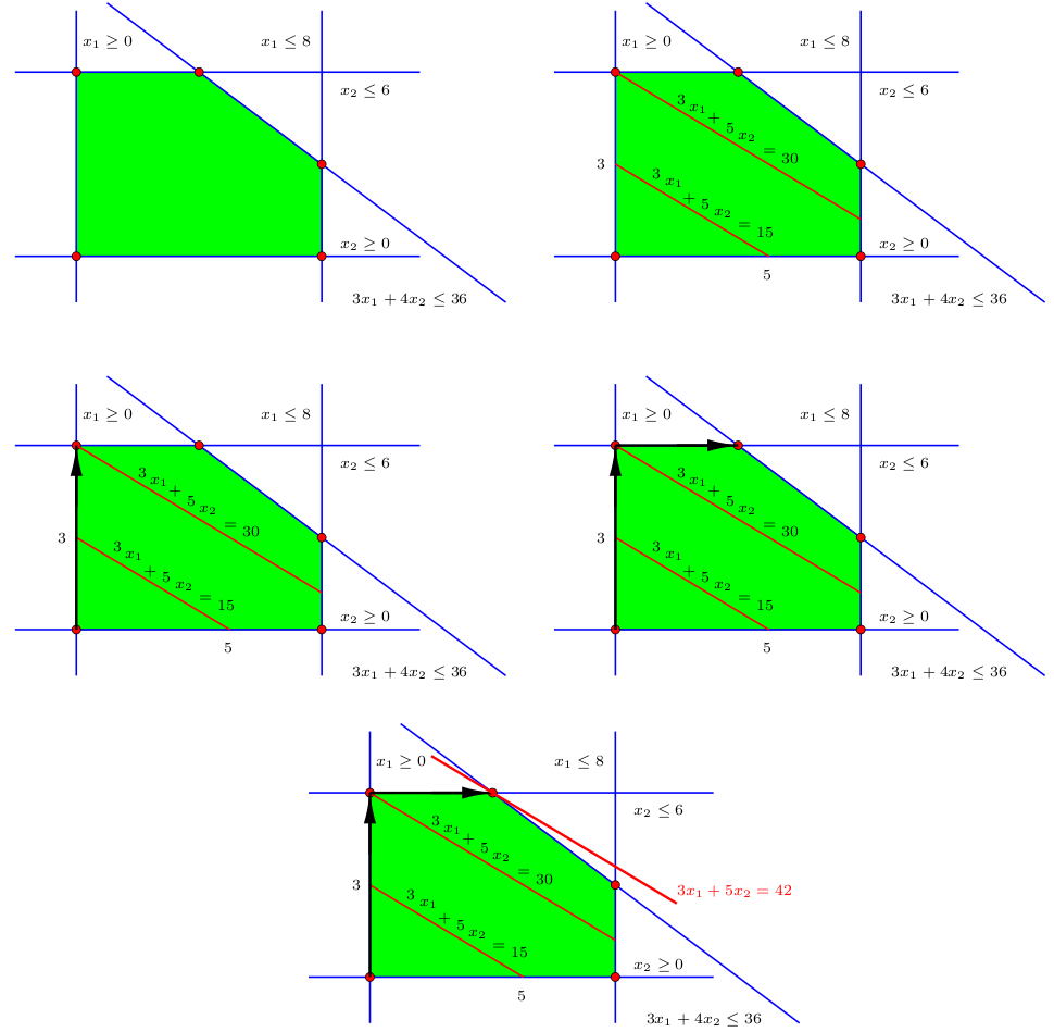
Fig. 45 The feasible region is bounded by the blue lines. All points on the red lines have the same value of the objective. We move from (0,0) to (0,6), and then to (4,6). At the optimal solution we can no longer increase the value of the objective.

Operations Research in Julia

• JuMP is a modeling language and collection of packages for mathematical optimization in Julia.

• GLPK is used for linear programming. GLPK is the GNU Linear Programming Kit, free software.

• The first tutorial is an example of the diet problem.

• Changhyun Kwon: Julia Programming for Operations Research, second edition. Free to read online, examples on github.

Duality

Every LP problem has a dual formulation and interpretation. Mathematically this is expressed as below:

\[\begin{split}\begin{array}{l} {\rm max}~{\displaystyle \sum_{j=1}^n c_j x_j} \\ {\rm subject~to} \\ \quad \left\{ \begin{array}{r} {\displaystyle \sum_{j=1}^n a_{ij} x_j \leq b_i},~~~ \\ {~}^{i = 1,2,\ldots,m} \\ x_j \geq 0, {~}_{j=1,2,\ldots,n} \end{array} \right. \end{array} \quad \quad \begin{array}{l} {\rm min}~{\displaystyle \sum_{i=1}^m b_i y_i} \\ {\rm subject~to} \\ \quad \left\{ \begin{array}{r} {\displaystyle \sum_{j=1}^m a_{ji} y_j \geq c_i},~~~ \\ {~}^{i = 1,2,\ldots,n} \\ y_j \geq 0, {~}_{j=1,2,\ldots,m} \end{array} \right. \end{array}\end{split}\]

The economic interpretation is as follows:

• \(x_j\) : level of activity \(j\),

• \(c_j\) : unit profit of activity \(j\),

• \(b_i\) : amount available of resource \(i\),

• \(a_{ij}\) : amount of resource \(i\) consumed by each unit of activity \(j\),

• \(y_i\) : contribution to profit per unit of resource \(i\).

The dual of our numerical example:

\[\begin{split}\begin{array}{l} \max 3 x_1 + 5 x_2 \\ \mbox{subject to} \\ \left\{ \begin{array}{l} \hphantom{3} x_1~ \hphantom{~+ 4 x_2} \leq 8 \\ \hphantom{3 x_1 + 4} x_2 \leq 6 \\ 3 x_1 + 4 x_2 \leq 36 \\ \hphantom{x_1 \geq 0,} ~x_1 \geq 0 \\ \hphantom{x_1 \geq 0,} ~x_2 \geq 0 \end{array} \right. \end{array} \quad \quad \mbox{is} \quad \quad \begin{array}{l} \min 8 y_1 + 6 y_2 + 36 y_3 \\ \mbox{subject to} \\ \left\{ \begin{array}{r} y_1 \hphantom{+ y_2} + 3 y_3 \geq 3 \\ \hphantom{y_1 +} y_2 + 4 y_3 \geq 5 \\ \hphantom{y_1 \geq 0,} ~y_1 \geq 0 \\ \hphantom{y_1 \geq 0,} ~y_2 \geq 0 \\ \hphantom{y_1 \geq 0,} ~y_3 \geq 0 \end{array} \right. \end{array}\end{split}\]

Shadow Prices

What are the units of the quantities in the dual problem? To introduce the notion of shadow price, let us consider a simplified model, the consumption of milk, using the following notations:

• \(c\) is the cost of one gallon milk,

• \(r\) is the nutritional requirement of calcium, and

• \(x\) is amount of milk consumed.

Then, our optimization problem is to determine \(x\) minimizing the cost, while satifying the nutritional requirement:

\[\min c x \quad \mbox{subject to} \quad a x \geq r.\]

What is \(a\)? Let us focus on the units. As the units of \(x\), the amount of milk consumed is gallons, and the unit of \(r\) is calcium we have

\[a = \frac{\mbox{calcium}}{\mbox{gallon}}\]

or, in words: \(a\) is is the amount of calcium in one gallon of milk.

While the primal minimizes the cost, the dual maximizes nutrients.

\[\max r y \quad \mbox{subject to} \quad a y \leq c.\]

What are the units of \(y\)? The unit of \(c\) is dollar, and recalling the units of \(a\), we derive

\[y = \frac{\mbox{dollar}}{\mbox{calcium}}.\]

Therefore, \(y\) is the cost of one unit of calcium. Then \(y\) is also called a shadow price.

Proposals of Project Topics

1. An industrial application.

   Read the paper by Ernest Koenigsberg: Some Industrial Applications of Linear Programming. Operational Research Society, Vol. 12, No. 2, pages 105-114, 1961.

   1. Select one problem and explain the LP formulation, in your own words.

   2. Work out an example with numerical data.

   3. Use JuMP to solve an instance of the same dimensions as in the paper.

   4. Report on the computational cost of the problem.

2. Managing a production facility.

   Read the first section of the book by Robert J. Vanderbei: Linear Programming. Foundations and Extensions. Fifth Edition, Springer-Verlag, 2020.

   1. Explain why the management of a production facility translates into an LP problem, in your own words.

   2. Setup a program to generate numerical data, for any dimension.

   3. Use JuMP to solve the generated instances.

   4. Report on the computational cost for various dimensions.

3. Solving network flow problems with JuMP.

   A network is a weighted directed graph allowing for flow to go from a source to a sink along the edges which each have a capacity.

   1. Starting with the JuMP tutorial on network flow problems, explore shortest path, assignment, and max-flow problems.

   2. Read the paper by Shuvomoy Das Gupta, J. Kevin Tobin, and Lacra Pavel on A two-step linear programming model for energy-efficient timetables in metro railway networks, in Transportation Research Part B, volume 93, pages 57-74, 2016.

   3. Explain the making of timetables as a network problem. Elaborate an illustrative example.

4. Simplex is not a polynomial-time algorithm.

   The title of this topic comes from the title of section 8.6 of the book Combinatorial Optimization. Algorithms and Complexity by Christos H. Papadimitriou and Kenneth Steiglitz, Dover 1998. Study also How good is the simplex algorithm? by Victor Klee and George J. Minty, in Inequalities III, pages 159-175, Academic Press, 1972.

   1. Formulate the construction of the Klee-Minty cube.

   2. Set up the formulation for any dimension to run experiments with the LP solver in GLPK.

   3. Do you observe exponential running times for increasing dimensions?

Exercises

1. Suppose General Motors makes a profit of \(\$100\) on each Chevrolet, \(\$200\) on each Buick, and \(\$400\) on each Cadillac.

   • These cars get 20, 17, and 14 miles a gallon respectively.

   • It takes respectively 1, 2, and 3 minutes to assemble one Chevrolet, one Buick, and one Cadillac.

   • Assume the company is mandated by the government that the average car has a fuel efficiency of at least 18 miles a gallon.

   Under these constraints, determine the optimal number of cars, maximizing the profit, which can be assembled in one 8-hour day. Formulate the linear programming problem.

2. Consider the diet problem, look at the tutorial example of JuMP.

   1. Write the dual of that example of the diet problem.

   2. What are the units of the dual variables?

3. Suppose an investor has a choice between three types of shares.

   Type A pays 4 percent, type B pays 6 percent, and type C pays 9 percent interest.

   The investor has \(\$100,000\) available to buy shares and wants to maximize the interest, under the following constraints:

   1. no more than \(\$20,000\) can be spent on shares of type C, and

   2. at least \(\$10,000\) should be spent on shares of type A.

   Answer the following questions:

   1. Give the mathematical description of the optimization problem.

   2. Bring the problem into the standard form.

   3. Solve the linear programming problem.

4. Suppose we have three machines \(m_1\), \(m_2\), \(m_3\), and three jobs \(j_1\), \(j_2\), \(j_3\).

   Each machine is capable to do all jobs, but the completion times are different for each machine, as expressed in the table below:

   \[\begin{split}\begin{array}{c|ccc} & j_1 & j_2 & j_3 \\ \hline m_1 & 4 & 3 & 9 \\ m_2 & 3 & 2 & 6 \\ m_3 & 9 & 5 & 7 \end{array}\end{split}\]

   The first row states that machine \(m_1\) does job \(j_1\) in 4 minutes, job \(j_2\) in 3 minutes, and job \(j_3\) in 9 minutes. Read the other rows similarly.

   The problem is to assign each machine to exactly one job, minimizing the sum of the completion times.

   Formulate this problem as a linear programming problem. Solve the problem. Verify that your formulation is correct.

5. The simplex algorithms performs very well on large problems, but in some cases an exponential number of vertices are visited, exponential in the number of equations and variables.

   Consider the sequences of vertices:

   \[\begin{split}\begin{array}{l} (\epsilon, \epsilon^2, \epsilon^3), (1, \epsilon, \epsilon^2), (1, 1-\epsilon,\epsilon-\epsilon^2), (\epsilon, 1-\epsilon^2, \epsilon -\epsilon^3), \\ (\epsilon, 1-\epsilon^2, 1 - \epsilon+\epsilon^3), (1 , 1-\epsilon, 1-\epsilon+\epsilon^2), (1, \epsilon, 1-\epsilon^2), \\ (\epsilon, \epsilon^2, 1-\epsilon^3), \mbox{ for } \epsilon: 0 < \epsilon < 1/2. \end{array}\end{split}\]

   1. Verify that maximizing the third coordinate \(x_3\), the vertices form an increasing sequence and that we visit all eight.

   2. Set up the linear programming problem and solve it.