Regression

We introduce regression from a linear algebra perspective.

Solving Overdetermined Linear Systems

Consider \(A {\bf x} = {\bf b}\), \(A\) is m-by-n, with \(m \geq n\). If \(m > n\), then we have more equations than unknowns and we can ask: How to solve this overdetermined linear system?

• As the overdetermined linear system has in many cases no exact solution, the problem of solving the system is reformulated into an optimization problem: Minimize \(\| {\bf b} - A {\bf x} \|_2^2\), or in words: solve the linear system in the least squares sence.

• To solve in the least square sense, the matrix \(A\) is factored into a product of an orthogonal matrix \(Q\) and and upper triangular matrix \(R\). A numerically stable algorithm to compute the QR decomposition is the Householder QR algorithm.

• While the Householder QR is a direct method to solve the least squares problem, for very large problems, an iterative algorithm such as the Generalized Minimum Residual Method is recommended.

• To verify a solution of a least squares problem, we exploit the orthogonality: \(\langle {\bf b} - A {\bf x} , A \rangle = 0\), which expresses that the residual vector \({\bf b} - A {\bf x}\) is perpendicular to the column space of the matrix \(A\).

• The solution of a least squares problem gives the coefficients of a data fit with a basis of polynomials, exponentials, or periodic functions.

The backslash operator applies to overdetermined systems, as illustrated in the Julia session below:

julia> A = rand(3,2); b = rand(3,1);

julia> x = A\b;

julia> r = b - A*x
3×1 Matrix{Float64}:
 -0.038628108251110294
  0.4381284983642053
 -0.17773235808476184

julia> r'*A
 1×2 Matrix{Float64}:
  -2.77556e-17  -2.77556e-17

The outcome of r'*A or \(\langle {\bf b} - A {\bf x} , A \rangle\) is below machine precision.

A typical application is to find a trend in numerical data.

• Input: \((x_i, y_i)\), \(i=1,2,\ldots,m\).

• Output: \((a, b)\), slope and intercept of a line \(y = a x + b\),

so that

\[\sum_{i=1}^m \left( \vphantom{\frac{1}{2}} y_i - (a x_i + b) \right)^2\]

is minimal. If the slope \(a\) is positive, then the trend in the data is increasing. In Fig. 46 is an illustration of fitting noisy data.

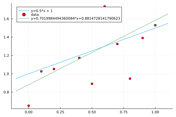
Fig. 46 Fitting data sampled from a line, with noise added.

The Julia code to make the plot in Fig. 46, for execution in a Jupyter notebook, is below:

using Plots
# plot the exact data on the line y = 0.5*x + 1
x = -0.1:0.1:1.1
y = 0.5*x .+ 1
plot(x,y,label="y=0.5*x + 1",legend=:topleft)
# add normally distributed noise
ynoisy = [y[i] + 0.2*randn() for i=1:length(y)]
scatter!(x[2:length(x)-1],ynoisy[2:length(x)-1],
         marker=(:red),label="data",legend=:topleft)
# set up the linear system
A = ones(length(x),2)
A[:,2] = x
# apply the backslash operator
c = A\ynoisy
# plot the fitted line
lbl = string("y=", string(c[2]), "*x+", string(c[1]))
fity = c[1] .+ c[2]*x
plot!(x,fity,label=lbl)

To fit exponential growth, linearization is applied. Given \((t_i, f_i)\), \(i=0,1,\ldots,n\), find the coefficients of

\[y(t) = c_1 e^{c_2 t} = c_1 \exp(c_2 t),\]

so \(y(t)\) fits the data \((t_i, f_i)\) best. With linearization, we consider

\[\ln(y(t)) = \ln(c_1 e^{c_2 t}) = \ln(c_1) + c_2 t.\]

The logarithmic scale helps to deal with numerical instabilities caused by extreme values which may arise with exponential growth.

Predictive Models

In statistical software, the least squares problem is known as the ordinary least squares. The Generalized Linear Model is abbreviated as GLM. An example from the GLM documentation is illustrated below.

julia> using DataFrames, GLM

julia> data = DataFrame(X=[1,2,3], Y=[2,4,7])
3x2 DataFrame
 Row  X      Y
      Int64  Int64

   1      1      2
   2      2      4
   3      3      7

For the give data, we define a linear model in the continuation of the Julia session:

julia> ols = lm(@formula(Y ~ X), data)
StatsModels.TableRegressionModel{
LinearModel{GLM.LmResp{Vector{Float64}},
GLM.DensePredChol{Float64,
LinearAlgebra.CholeskyPivoted{Float64,
Matrix{Float64}}}}, Matrix{Float64}}

Y ~ 1 + X

Coefficients:

                 Coef.  Std. Error

(Intercept)  -0.666667    0.62361
X             2.5         0.288675

As an application of the least squares model, we can predict data.

julia> predict(ols)
3-element Vector{Float64}:
 1.8333333333333308
 4.333333333333334
 6.833333333333336

julia> line(x) = -2/3 + 2.5*x
line (generic function with 1 method)

julia> [line(t) for t in [1,2,3]]
3-element Vector{Float64}:
 1.8333333333333335
 4.333333333333333
 6.833333333333333

Recall an earlier lecture analyzing data and the question Are the winters in Chicago becoming milder? To answer this question, we obtained data from the National Weather Service, a site from the National Oceanic and Atmospheric Administration (NOAA). The data are average monthly temperatures in Chicago over the past 100 years, from 1922 to 2021. The file tempChicago100years.txt stores the data.

The Julia code in the Jupyter notebook loads the data and makes a plot, shown in Fig. 47.

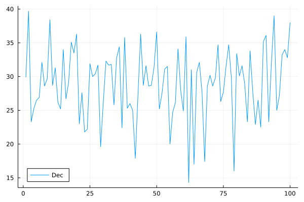
Fig. 47 Average December temperatures in Chicago from 1922 to 2021.

using DelimitedFiles
A = readdlm("tempChicago100years.txt")
dectemp = A[2:end,13]
plot(1:100, dectemp, label="Dec", legend=:bottomleft)

The code in the Jupyter notebook continues with the preparation of the data for the fit. The type of the elements in the matrix A is Any, which then causes problems later, so we must convert to Float64.

years = A[2:end,1]
tempdf = DataFrame(X=Vector{Float64}(years),
                   Y=Vector{Float64}(dectemp))

The command olstemp = lm(@formula(Y ~ X), tempdf) fits the average December temperatures, and gives the output:

Y ~ 1 + X

Coefficients:
---------------------------------
                Coef.  Std. Error
---------------------------------
(Intercept)  20.4113      35.8233
X             0.00433003   0.0181687

Observe that the slope 0.00433 is tiny … which becomes apparent in the plot in Fig. 48.

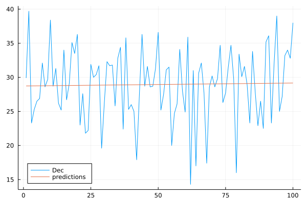
Fig. 48 A linear fit of the average December temperatures.

To make the plot, we grab the coefficients of the fit:

cff = coef(olstemp)

and then compute the predictions:

predicted = [cff[1] + cff[2]*t for t in 1922:2021]

and plot for the same range 1:100 as the December temperatures:

plot!(1:100, predicted, label="predictions")

Instead of making the fit for the entire 100 years, let us look at the last 20 years, done by the code below:

Xlast20=Vector{Float64}(years[end-19:end])
Ylast20=Vector{Float64}(dectemp[end-19:end])
tempdf20 = DataFrame(X=Xlast20,Y=Ylast20)
olstemp20 = lm(@formula(Y ~ X), tempdf20)
cff20 = coef(olstemp20)

The coefficients are

-607.1678947233604
   0.3168421052564556

The larger slope 0.316 is noticeable in Fig. 49.

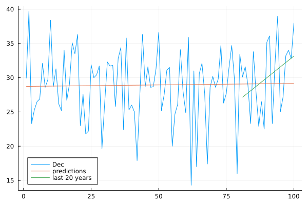
Fig. 49 A linear fit of the average December temperatures, over the last 20 years.

Regression as a Data Mining Task

Definition of Regression as a Data Mining Task.

In the modeling view of data mining, regression is a task of predicting a numeric target attribute which represents some quantity of interest.

This quantity of interest could be

• an outcome or a parameter of an industrial process,

• an amount of money earned or spent,

• a cost or gain due to a business decision, etc.

Data mining has its origins in machine learning and statistics. In data mining: domain, instance, attribute, and dataset. In statistics: population, observation, variable, and sample are the respective counterparts to the data mining terms.

Proposals of Project Topics

1. Fit census data.

   Using census data from 1790 to today, find experimentally a best fitting polynomial for the U.S. population in millions against time in decades. Consider the following questions:

   • What is the best degree of polynomial?

   • Instead of one single polynomial, would a piecewise polynomial model fit better?

2. Fit corona virus data.

   Use data from the covid-19 pandemic to model the exponential growth in a surge of infections. Consider the following questions:

   • What is the exponent in the surge?

   • Do different surges have different exponents?

Exercises

1. Does Moore’s Law still hold? The data in Table 1 are taken from wikipedia.

   Table 1 Transistor counts for various Intel processors.

   year	Intel processor	transistor count
   2000	Pentium III Coppermine	21,000,000
   2001	Pentium III Tualatin	45,000,000
   2002	Pentium IV Northwood	55,000,000
   2003	Itanium 2 Madison	410,000,000
   2004	Itanium 2	592,000,000
   2005	Pentium D Smithfield	228,000,000
   2006	Dual-core Itanium 2	1,700,000,000
   2007	Core 2 Duo Wolfdale	411,000,000
   2008	Core i7 quad-core	731,000,000
   2010	Xeon Nehalem-EX (8-core)	2,300,000,000

   Fit the data in Table 1 to \(y(t) = c_1 2^{c_2 t}\).

   Make a \(\log_2\) scale plot: \((\mbox{year}, \log_2(\mbox{transistor count}))\) of the data, and the model \(y(t)\). For year, use 0, 1, \(\ldots\), 10.

2. Complete the plot in Fig. 49 with the fit for the last 20 years with the fits for 1922-1941, 1942-1961, 1962-1981, and 1982-2001.

3. Adjust the code of the previous exercise, so that instead of 20, any divisor of 100 could be used to break up the data.

Bibliography

1. Jose Storopoli, Rik Huijzer, Lazaro Alonso: Julia Data Science. First edition published 2021. <https://juliadatascience.io> Creative Commons Attribution-Noncommercial-ShareAlike 4.0 International.

2. Pawel Cichosz: Data Mining Algorithms: Explained Using R. Wiley 2015.