Least Squares Chebyshev and Fourier

We consider the problem of approximating functions twice: once with a basis of Chebyshev polynomials, and once with a basis of Fourier series.

Approximating Functions with Orthogonal Bases

Consider an interval \([a,b]\) and a basis of functions \(\phi_i\), \(i=0,1,2,\ldots\), equipped with an inner product:

\[\langle f, g \rangle,\]

for any pair of functions \(f\) and \(g\). If for the basis functions \(\phi_i\) we have

\[\begin{split}\langle \phi_i , \phi_j \rangle = \left\{ \begin{array}{ll} 0, & i \not= j, \\ 1, & i = j. \end{array} \right.\end{split}\]

then we say that the basis \(\{ \phi_0, \phi_1, \phi_2, \ldots \}\) is orthogonal.

For any function \(f(x)\) over \([a,b]\), consider the series

\[f(x) = \sum_{i=0}^\infty c_i \phi_i(x), \quad c_i = \langle f, \phi_i \rangle.\]

Truncate the series to the first \(n+1\) terms:

\[f(x) = p(x) + \sum_{i=n+1}^\infty c_i \phi_i(x), \quad \mbox{with} \quad p(x) = \sum_{i=0}^n c_i \phi_i(x).\]

Because \(c_i = \langle f, \phi_i \rangle\) and \(\phi_i\) is an orthogonal basis:

\[\langle f - p, \phi_i \rangle = 0, \quad i=0,1,\ldots,n,\]

and therefore \(p\) is the least squares approximation for \(f\).

Chebyshev Approximations

Definition of the Chebyshev polynomial.

The Chebyshev polynomial \(T_n(x)\) is \(\cos(n \arccos(x))\).

From the definition of the Chebyshev polynomial it is not immediately obvious that \(T_n(x)\) is a polynomial. Chebyshev polynomials can be computed via the recursion:

\[T_0(x) = 1, \quad T_1(x) = x, \quad T_n(x) = 2x T_{n-1}(x) - T_{n-2}(x).\]

Now we can verify that for the base cases of the recursion, we obtain polynomials: \(T_0(x) = \cos(0) = 1\), \(T_1(x) = \cos( \arccos(x)) = x\).

For general degree \(n\), consider the identities:

\[\begin{split}\begin{array}{ccrcccc} & & \cos(a + b) & = & \cos(a) \cos(b) & + & \sin(a) \sin(b) \\ + & & \cos(a - b) & = & \cos(a) \cos(b) & - & \sin(a) \sin(b) \\ \hline \multicolumn{3}{c}{\cos(a+b) + \cos(a-b)} & = & 2 \cos(a) \cos(b) \end{array}\end{split}\]

Apply the above identity to \(a = n \arccos(x)\), \(b = \arccos(x)\).

Any polynomial can be written in the Chebyshev polynomial basis. Consider \(T_{n+1}(x) = 2x T_n(x) - T_{n-1}(x)\), \(T_0(x) = 1\), \(T_1(x) = x\). Writing out the first six polynomials, in expanded form:

\[\begin{split}\begin{array}{l} T_0(x) = 1 \\ T_1(x) = x \\ T_2(x) = 2 x^2 - 1 \\ T_3(x) = 4 x^3 - 3 x \\ T_4(x) = 8 x^4 - 8 x^2 + 1 \\ T_5(x) = 16 x^5 - 20 x^3 + 5x \end{array}\end{split}\]

and rearranging in matrix-vector notation gives:

\[\begin{split}\left[ \begin{array}{c} T_0 \\ T_1 \\ T_2 \\ T_3 \\ T_4 \\ T_5 \end{array} \right] = \left[ \begin{array}{cccccc} 1 & 0 & 0 & 0 & 0 & 0 \\ 0 & 1 & 0 & 0 & 0 & 0 \\ -1 & 0 & 2 & 0 & 0 & 0 \\ 0 & -3 & 0 & 4 & 0 & 0 \\ 1 & 0 & -8 & 0 & 8 & 0 \\ 0 & 5 & 0 & -20 & 0 & 16 \end{array} \right] \left[ \begin{array}{c} 1 \\ x \\ x^2 \\ x^3 \\ x^4 \\ x^5 \end{array} \right].\end{split}\]

Observe that the lower triangular matrix is invertible. Using the inverse of the above matrix, any polynomial of degree 5 or less can can be written as a linear combination of Chebyshev polynomials. This shows that we have a basis of polynomials.

The Chebyshev basis is orthogonal with respect to the inner product

\[\langle f , g \rangle = \frac{2}{\pi} \int_{-1}^{+1} \frac{f(x) g(x)}{\sqrt{1 - x^2}} dx.\]

For the Chebyshev polynomials \(T_i\), we have

\[\begin{split}\langle T_i , T_j \rangle = \left\{ \begin{array}{ll} 0, & i \not= j, \\ 1, & i = j. \end{array} \right.\end{split}\]

Therefore, the Chebyshev polynomials form an orthogonal basis.

We can approximate any function \(f\) with a Chebyshev series:

\[f(x) = \frac{c_0}{2} + \sum_{i=1}^\infty c_i T_i(x) = p(x) + \sum_{i=n+1}^\infty c_i T_i(x), \quad {\rm with}~ c_i = \langle f , T_i \rangle,\]

for \(i=0,1,\ldots,n\), where

\[p(x) = \frac{c_0}{2} + \sum_{i=1}^n c_i T_i(x),\]

is the truncation of the Chebyshev series.

By construction: \(\langle f - p, T_i \rangle = 0\), \(i=0,1,\ldots,n\). The polynomial \(p\) is a least squares approximation for \(f\).

The Julia function below defines an array of basis functions.

"""
   function basis(n::Int64)

returns an array of functions with the first n
Chebyshev polynomials.
"""
function basis(n::Int64)
   t0(x) = 1
   result = [t0]
   if(n > 1)
      t1(x) = x
      result = [result; t1]
      t1two(x) = 2*x
      for i=3:n
          newt(x) = t1two(x)*result[i-1](x) - result[i-2](x)
          result = [result; newt]
      end
    end
    return result
end

The function basis is then used to make the plot in Fig. 50.

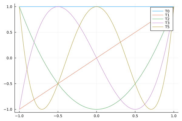
Fig. 50 The first five Chebyshev polynomials.

We compute the inner product via Gauss-Chebyshev quadrature:

\[\langle f , g \rangle = \frac{2}{\pi} \int_{-1}^{+1} \frac{f(x) g(x)}{\sqrt{1 - x^2}} dx\]

as defined in the function innerproduct below:

using FastGaussQuadrature

nodes, weights = gausschebyshev(16)
rule(f) = sum([weights[k]*f(nodes[k]) for k=1:length(weights)])

"""
    function innerproduct(f::Function, g::Function)

returns the value of the inner product of the functions f and g,
by the integral of f and g over [-1,+1] with weight 1/sqrt(1-x^2).
"""
function innerproduct(f::Function, g::Function)
   fun(x) = f(x)*g(x)
   return (2.0/pi)*rule(fun)
end

Verifying the orthogonality of the basis, all inner products for the first five basis functions \(T_i\), \(i=0,1,2,3,4\), at row \(i\) and column \(j\) is the value of \(\langle T_i, T_j \rangle\):

+2.00e+00 +1.06e-16 -5.30e-17 +1.06e-16 -7.07e-17
+1.06e-16 +1.00e+00 +1.59e-16 -8.83e-17 +2.65e-16
-5.30e-17 +1.59e-16 +1.00e+00 +3.00e-16 -2.12e-16
+1.06e-16 -8.83e-17 +3.00e-16 +1.00e+00 +3.71e-16
-7.07e-17 +2.65e-16 -2.12e-16 +3.71e-16 +1.00e+00

We observe the identity matrix (modulo roundoff of machine precision), except for the first number in the first row and column, which equals 2.

The coefficients of the Chebyshev approximant are computed with respect to the basis. The Julia function coefficients computes \(\langle f, T \rangle\) for all \(T\) in the basis.

"""
    function coefficients(f::Function,b::Array{Function,1})

returns the inner products of f with the basis functions in b.
"""
function coefficients(f::Function,b::Array{Function,1})
   dim = length(b)
   result = zeros(dim)
   for i=1:dim
       result[i] = innerproduct(f,b[i])
   end
   return result
end

As an illustration, we compute a cubic approximation for \(\exp\):

\[p(x) = \frac{c_0}{2} + \sum_{i=1}^n c_i T_i(x), \quad c_i = \langle \exp, T_i \rangle, \quad i = 0,1,\ldots,n.\]

The cubic least squares approximant for \(\exp(x)\) is shown in Fig. 51.

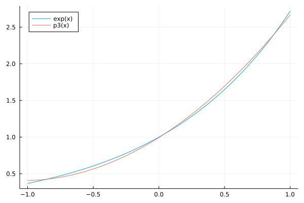
Fig. 51 A Chebyshev approximation for \(exp(x)\) of degree 3.

The error of the cubic least squares approximant is shown in Fig. 52.

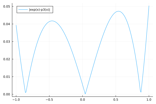
Fig. 52 The error of the cubic least squares approximant of \(exp(x)\).

Fitting Functions with Fourier Series

Many functions are periodic and to fit those functions, we use an orthogonal trigonometric basis. Starting with the constant function 1, we consider sine and cosine functions with increasing frequency, respectively \(\sin(k \pi t)\) and \(\cos(k \pi t)\), for \(k = 1,2,\ldots,n\). With respect to the inner product

\[\langle f , g \rangle = \int_{-1}^{+1} f(t) g(t) dt,\]

the functions in the basis are orthogonal to each other. For any \(k\) and \(\ell\): \(\langle \sin(k \pi t), \cos(\ell \pi t) \rangle = 0\) and

\[\begin{split}\langle \sin(k \pi t), \sin(\ell \pi t) \rangle = \left\{ \begin{array}{ll} 0, & k \not= \ell, \\ 1, & k = \ell. \end{array} \right.\end{split}\]

The same holds for the cosine functions.

The least squares approximation for any function \(f(t)\) for \(t \in [-1,+1]\) is then

\[p(t) = \frac{a_0}{2} + \sum_{k=1}^n \left( \vphantom{\frac{a_0}{2}} a_k \cos(k \pi t) + b_k \sin(k \pi t) \right),\]

where the coefficients are computed as

\[a_0 = \langle f, 1 \rangle, \quad a_k = \langle f, \cos(k \pi t) \rangle, \quad b_k = \langle f, \sin(k \pi t) \rangle.\]

Because of the orthogonal basis \(f-p\) is orthogonal to the basis and \(p\) is the least squares approximation for \(f\).

For the interval \([0,1]\), instead of \([-1,+1]\), consider the basis functions \(\cos(k 2 \pi t)\) and \(\sin(k 2 \pi t)\), \(k=1,2,\ldots\)

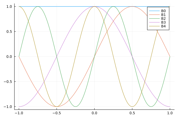
Fig. 53 The first five functions in the Fourier basis.

The first five basis functions shown in Fig. 53 uses the Julia function to define an array of basis functions. The basis functions are 1, \(\cos(k \pi t)\), and \(\sin(k \pi t)\), for \(k = 1,2,\ldots,n\).

"""
    function basis(n::Int64)

returns an array of functions with
the first 2*n+1 basis polynomials.
"""
function basis(n::Int64)
    one = [(t) -> 1]
    sines = [(t) -> sin(k*pi*t) for k=1:n]
    cosines = [(t) -> cos(k*pi*t) for k=1:n]
    result = [one; sines; cosines]
    return result
end

The inner product is computed via Gauss-Legendre quadrature:

\[\langle f , g \rangle = \int_{-1}^{+1} f(x) g(x) dx.\]

and with the Julia code below:

using FastGaussQuadrature

nodes, weights = gausslegendre(32)
rule(f) = sum([weights[k]*f(nodes[k]) for k=1:length(weights)])

"""
    function innerproduct(f::Function, g::Function)

returns the value of the inner product of the functions f and g,
by the integral of f and g over [-1,+1].
"""
function innerproduct(f::Function, g::Function)
   fun(x) = f(x)*g(x)
   return rule(fun)
end

To verify the orthogonality of the basis, we compute all inner products for the first five basis functions \(B_i\), \(i=0,1,2,3,4\), at row \(i\) and column \(j\) is the value of \(\langle B_i, B_j \rangle\):

+2.00e+00 +6.26e-17 +5.57e-17 +4.46e-16 -1.04e-16
+6.26e-17 +1.00e+00 +1.93e-16 +2.79e-17 -1.78e-17
+5.57e-17 +1.93e-16 +1.00e+00 -3.37e-17 -5.71e-18
+4.46e-16 +2.79e-17 -3.37e-17 +1.00e+00 +2.93e-16
-1.04e-16 -1.78e-17 -5.71e-18 +2.93e-16 +1.00e+00

We observe the identity matrix (modulo roundoff of machine precision), except for the first number in the first row and column, which equals 2.

As an example of fitting a periodic function, consider \(f(t) = (\sin(2 \pi t))^3\), for \(t \in [-1,+1]\). We compute the coefficients

\[a_0 = \langle f, 1 \rangle, \quad a_k = \langle f, \cos(k \pi t) \rangle, \quad b_k = \langle f, \sin(k \pi t) \rangle\]

of

\[p(t) = \frac{a_0}{2} + \sum_{k=1}^n \left( \vphantom{\frac{a_0}{2}} a_k \cos(k \pi t) + b_k \sin(k \pi t) \right),\]

for

• \(n = 3\) (7 basis functions), shown in Fig. 54 (with error in Fig. 55) and

• \(n = 6\) (13 basis functions), shown in Fig. 56.

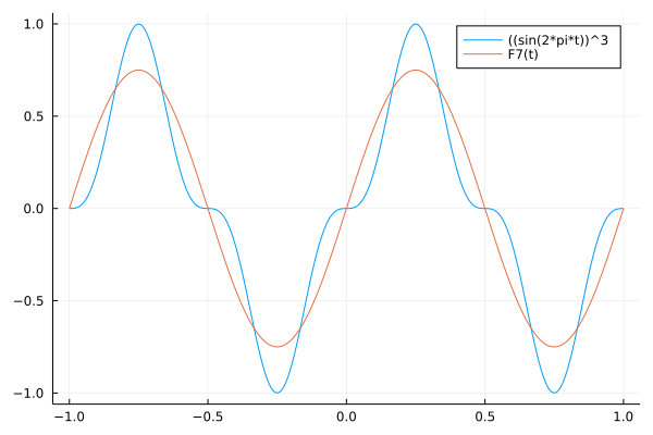
Fig. 54 The approximation with 7 basis functions.

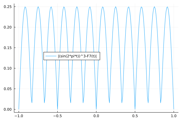
Fig. 55 The error of the approximation with 7 basis functions.

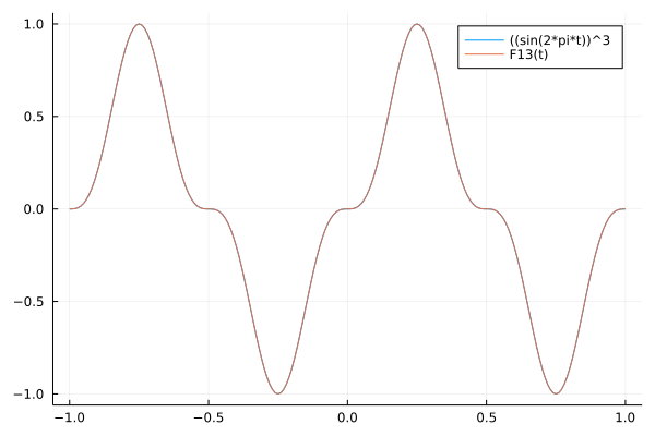
Fig. 56 The approximation with 13 basis functions.

Looking at the Fourier series representation, for \(n = 6\) (13 basis functions), only two coefficients are nonzero:

1. \(0.75\) at index 3, and

2. \(-0.25\) at index 7.

These two indices respectively correspond to \(\sin(2 \pi t)\) and \(\cos(\pi t)\). Therefore, we can write

\[\left( \vphantom{\frac{3}{4}} \sin(2\pi t) \right)^3 = \frac{3}{4} \sin(2 \pi t) - \frac{1}{4} \cos(\pi t).\]

This symbolic result is shown in Fig. 57.

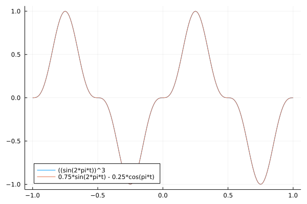
Fig. 57 A symbolic result of a Fourier approximation.

Proposals of Project Topics

1. Fit average daily temperatures.

   Obtain the average temperature for each day of one year. Fit the data with a trigonometric basis.

   Consider the following questions:

   • How large should the basis be for an accurate representation?

   • Compare the fit of one year on data of another year.

     How good does the fit predict the temperature of the other year?

2. On the origin of the Chebyshev polynomials

   How did Chebyshev arrive at his polynomials? Consider the paper by V. L. Goncharov: The Theory of Best Approximation of Functions. Journal of Approximation Theory 106:2–57, 2000.

   The second section of this paper describes the memoir Theorie des mecanismes connus sous le nom de parallelogrammes, by Chebyshev, which appeared in 1854.

   Consider the following questions:

   • Verify the reduction of computing a best approximating polynomial to a differential equation.

   • Illustrate your verification with some computational experiments.

Exercises

1. Consider the approximation of \(\exp(x)\) by Chebyshev polynomials.

   How large should the degree of the approximant be for the largest error to be less than \(10^{-6}\) over \([-1,+1]\)?

2. Consider \(f(x) = 4 \sin(2 \pi x) + 3 \sin(5 \pi x)\) over \([-1,+1]\).

   Compute a Chebyshev approximation with a high enough degree so the error is below \(10^{-6}\) for all \(x \in [-1,+1]\).

3. Consider \(f(x) = 4 \sin(2 \pi x) + 3 \sin(5 \pi x)\) over \([-1,+1]\).

   • How many terms in the trigonometric basis are needed to represent \(f\)? Verify this numerically.

   • Compare with the outcome of Exercise 2. Which method, Chebyshev polynomials or Fourier series, is preferred for this \(f\).

4. Consider Fourier series approximations for \(\exp(x)\) over \([-1,+1]\).

   • How many terms in the Fourier series are needed for the largest error in the approximation to be less than \(10^{-6}\)?

   • Compare with the outcome of Exercise 1. Which method, Chebyshev polynomials or Fourier series, is preferred for \(\exp(x)\)?